Summary
The following tutorial introduces the use of an autoregressive model for generating sequences of dance poses. This model extends the model introduced in an earlier article in that it combines a long short term memory (LSTM) network with a mixture density network (MDN). A MDN outputs the parameters for multiple gaussian distributions. In the autoregressive model employed here, each gaussian distribution can be sampled from to obtain one candidate pose for continuing a pose sequence.
This tutorial forms part of a series of tutorials on using PyTorch to create and train generative deep learning models. The code for these tutorials is available here.
After 1000 epochs of training, the model generates pose sequences that look like this when rendered as skeleton animations.
Mixture Density Networks
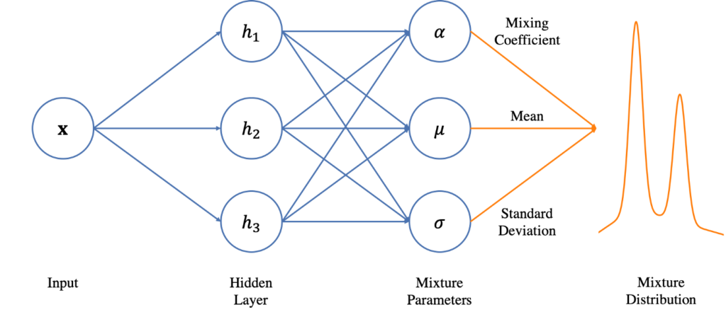
The conventional autoregressive model employed in the previous article predicts the continuation of a sequence as a deterministic output. This is problematic since many sequences are probabilistic in nature. Accordingly, their predicted continuation involves uncertainty. MDNs allow to take this into account by treating each feature of the predicted output as a random variable. They do so by outputting for every feature the parameters for a probability distribution. An actual value for the feature can then be obtained by sampling from the probability distribution. The term “Mixture Density” refers to the fact that a complicated probability distribution can be created by combining (“mixing”) multiple simple probability distributions. The simple distributions are typically Gaussian distributions. The MDN generates for each feature a predefined number of Gaussian distributions for each of which it outputs its parameters (mean and standard deviation) and mixing coefficient. Training involves approximating the true probability distributions of the features by tuning the Gaussian parameters and mixing coefficients.
From an application point of view, the addition of an MDN to an autoregressive model leads to a predicted sequence continuation that is less likely to stagnate after a few iterations than is the case with a conventional autoregressive model.
Create Model
This article skips an explanation of the code that deals with importing python modules and motion capture data and creating datasets, since all these steps are identical with the ones that have been explained previously.
The model that is created consists of two networks. A first network that consists of LSTM layers and a second network that operates as MDN. The first network takes as input a sequence of poses. Its output is then used as input for the MDN. The MDN outputs three tensors, one for each of the following parameters of a mixture of Gaussian distributions: mean values (mu), standard deviations (sigma), and mixture coefficients (alpha).
The MDN is implemented as a conventional artificial neural network. In this network, all layers except the last one are shared when creating the three output tensors. The last layer is split into three separate layers, one for each parameter of the distributions. The last layer that outputs the mixing coefficients employs an activation function, the others don’t. This activation function is Softmax to ensure that all mixing coefficients sum up to one. Another difference between the three last layers is their number of output dimensions. The layers that output mean and sigma values do so for each pose dimension and Gaussian distribution. The layer that outputs the mixing coefficients only outputs one value per Gaussian distribution.
The model is implemented by subclassing the nn.Module class. The class definition is as follows:
class AutoRegressor(nn.Module):
    def __init__(self, pose_dim, rnn_layer_count, rnn_layer_size, dense_layer_sizes, mix_count):
        super(AutoRegressor, self).__init__()

        self.pose_dim = pose_dim
        self.rnn_layer_count = rnn_layer_count
        self.rnn_layer_size = rnn_layer_size
        self.dense_layer_sizes = dense_layer_sizes
        self.mix_count = mix_count

        # create recurrent layers
        rnn_layers = []

        rnn_layers.append(("autoreg_rnn_0", nn.LSTM(self.pose_dim, self.rnn_layer_size, self.rnn_layer_count, batch_first=True)))
        self.rnn_layers = nn.Sequential(OrderedDict(rnn_layers))

        # create dense layers
        dense_layers = []
        dense_layer_count = len(self.dense_layer_sizes)

        if dense_layer_count > 0:
            dense_layers.append(("autoreg_dense_0", nn.Linear(self.rnn_layer_size, self.dense_layer_sizes[0])))
            dense_layers.append(("autoreg_dense_relu_0", nn.ReLU()))

            for layer_index in range(1, dense_layer_count):
                dense_layers.append( ("autoreg_dense_{}".format( layer_index ), nn.Linear( self.dense_layer_sizes[ layer_index - 1 ], self.dense_layer_sizes[ layer_index ] ) ) )
                dense_layers.append( ("autoreg_dense_relu_{}".format( layer_index ), nn.ReLU() ) )

            dense_layers.append( ("autoregr_dense_{}".format( len(self.dense_layer_sizes) ), nn.Linear( self.dense_layer_sizes[-1], self.pose_dim) ) )
        else:
            dense_layers.append(("autoreg_dense_0", nn.Linear(self.rnn_layer_size, self.pose_dim)))

        self.dense_layers = nn.Sequential(OrderedDict(dense_layers))

        # mdn mu layers
        mdn_mu_layers = []
        mdn_mu_layers.append(("autoreg_mdn_mu_dense", nn.Linear(self.pose_dim, self.pose_dim * self.mix_count)))
        self.mdn_mu_layers = nn.Sequential(OrderedDict(mdn_mu_layers))

        # mdn sigma layers
        mdn_sigma_layers = []
        mdn_sigma_layers.append(("autoreg_mdn_sigma_dense", nn.Linear(self.pose_dim, self.pose_dim * self.mix_count)))
        self.mdn_sigma_layers = nn.Sequential(OrderedDict(mdn_sigma_layers))

        # mdn alpha layers
        mdn_alpha_layers = []
        mdn_alpha_layers.append(("autoreg_mdn_alpha_dense", nn.Linear(self.pose_dim, self.mix_count)))
        mdn_alpha_layers.append(("autoreg_mdn_alpha_softmax", nn.Softmax(dim=1)))
        self.mdn_alpha_layers = nn.Sequential(OrderedDict(mdn_alpha_layers))

    def forward(self, x):
        #print("x 1 ", x.shape)
        x, (_, _) = self.rnn_layers(x)
        #print("x 2 ", x.shape)
        x = x[:, -1, :] # only last time step
        #print("x 3 ", x.shape)
        x = self.dense_layers(x)
        #print("x ", x.shape)
        mu = self.mdn_mu_layers(x)
        mu = mu.view((-1, self.mix_count, self.pose_dim))
        #print("mus ", mus.shape)
        sigma = self.mdn_sigma_layers(x)
        sigma = torch.exp(sigma)
        sigma = sigma.view((-1, self.mix_count, self.pose_dim))
        #print("sigmas ", sigmas.shape)
        alpha = self.mdn_alpha_layers(x)
        alpha = alpha.view((-1, self.mix_count))
        #print("alphas ", alphas.shape)
        return mu, sigma, alpha
The constructor of the model class takes the following arguments: the dimension of a single pose, the number of recurrent layers to create, the number of units in each LSTM layer, a list of units per layer in the artificial neural network that follows the LSTM network, and the number of Gaussian distributions. The model class can be instantiated as follows:
ar_rnn_layer_count = 2
ar_rnn_layer_size = 512
ar_dense_layer_sizes = [ ]
ar_mdn_mix_count = 4

autoreg = AutoRegressor(pose_dim, ar_rnn_layer_count, ar_rnn_layer_size, ar_dense_layer_sizes, ar_mdn_mix_count).to(device)
The shapes of the input and output tensors for this model are as follows:
- input tensor: batch_size x sequence_length x pose_dim
- output tensor mu: batch_size x pose_dim * mixture count
- output tensor sigma: batch_size x pose_dim * mixture count
- output tensor alpha: batch_size x mixture count
Optimiser and Loss Functions
The loss function that has been previously used to calculate the reconstruction error between the target and predicted joint rotations is replaced here by a new loss function. This function is named “mdn_loss” and calculates the loss based on the negative log likelihood of obtaining the correct target features when sampling from the current mixture distribution. The negative log likelihood is a common measure for calculating the error of probabilistic models. The reason why a negative log likelihood is used instead of a direct probability is as follows: logarithms are mathematically easier to deal with since multiplication become additions and divisions become subtractions, and since gradient descent minimises a loss, the log likelihood has to be made negative.
The “mdn_loss” function is implemented as follows:
def mdn_loss(y, mu, sigma, alpha):
    """Calculates the error, given the MoG parameters and the target
    The loss is the negative log likelihood of the data given the MoG
    parameters.
    """
    normal = Normal(mu, sigma+1e-7) # avoid a standard deviation of zero
    loglik = normal.log_prob(y.expand_as(sigma))

    loglik = torch.mean(loglik, dim=2)
    loss = -torch.logsumexp(torch.log(alpha) + loglik, dim=1)

    return torch.mean(loss)
The overall loss function is now as follows:
def ar_loss(y, mu, sigma, alpha):

    _norm_loss = ar_norm_loss(mu)
    _mdn_loss = mdn_loss(y, mu, sigma, alpha)

    #print("_mdn_loss ", _mdn_loss)

    _total_loss = 0.0
    _total_loss += _norm_loss * ar_norm_loss_scale
    _total_loss += _mdn_loss * ar_mdn_loss_scale

    return _total_loss, _norm_loss, _mdn_loss
Training and Testing Functions
The functions for training and testing differ minimally from their implementations in the previous article:
def ar_train_step(pose_sequences, target_poses):

    mu, sigma, alpha = autoreg(pose_sequences)

    _ar_loss, _ar_norm_loss, _ar_mdn_loss = ar_loss(target_poses, mu, sigma, alpha)

    #print("_ae_pos_loss ", _ae_pos_loss)

    # Backpropagation
    ar_optimizer.zero_grad()
    _ar_loss.backward()

    ar_optimizer.step()

    return _ar_loss, _ar_norm_loss, _ar_mdn_loss

def ar_test_step(pose_sequences, target_poses):

    autoreg.eval()

    with torch.no_grad():
        mu, sigma, alpha = autoreg(pose_sequences)
        _ar_loss, _ar_norm_loss, _ar_mdn_loss = ar_loss(target_poses, mu, sigma, alpha)

    autoreg.train()

    return _ar_loss, _ar_norm_loss, _ar_mdn_loss

def train(train_dataloader, test_dataloader, epochs):

    loss_history = {}
    loss_history["ar train"] = []
    loss_history["ar test"] = []
    loss_history["ar norm"] = []
    loss_history["ar mdn"] = []

    for epoch in range(epochs):
        start = time.time()

        ar_train_loss_per_epoch = []
        ar_norm_loss_per_epoch = []
        ar_mdn_loss_per_epoch = []

        for train_batch in train_dataloader:
            input_pose_sequences = train_batch[0].to(device)
            target_poses = train_batch[1].to(device)

            _ar_loss, _ar_norm_loss, _ar_mdn_loss = ar_train_step(input_pose_sequences, target_poses)

            _ar_loss = _ar_loss.detach().cpu().numpy()
            _ar_norm_loss = _ar_norm_loss.detach().cpu().numpy()
            _ar_mdn_loss = _ar_mdn_loss.detach().cpu().numpy()

            ar_train_loss_per_epoch.append(_ar_loss)
            ar_norm_loss_per_epoch.append(_ar_norm_loss)
            ar_mdn_loss_per_epoch.append(_ar_mdn_loss)

        ar_train_loss_per_epoch = np.mean(np.array(ar_train_loss_per_epoch))
        ar_norm_loss_per_epoch = np.mean(np.array(ar_norm_loss_per_epoch))
        ar_mdn_loss_per_epoch = np.mean(np.array(ar_mdn_loss_per_epoch))

        ar_test_loss_per_epoch = []

        for test_batch in test_dataloader:
            input_pose_sequences = train_batch[0].to(device)
            target_poses = train_batch[1].to(device)

            _ar_loss, _, _ = ar_train_step(input_pose_sequences, target_poses)

            _ar_loss = _ar_loss.detach().cpu().numpy()

            ar_test_loss_per_epoch.append(_ar_loss)

        ar_test_loss_per_epoch = np.mean(np.array(ar_test_loss_per_epoch))

        if epoch % model_save_interval == 0 and save_weights == True:
            autoreg.save_weights("results/weights/autoreg_weights_epoch_{}".format(epoch))

        loss_history["ar train"].append(ar_train_loss_per_epoch)
        loss_history["ar test"].append(ar_test_loss_per_epoch)
        loss_history["ar norm"].append(ar_norm_loss_per_epoch)
        loss_history["ar mdn"].append(ar_mdn_loss_per_epoch)

        print ('epoch {} : ar train: {:01.4f} ar test: {:01.4f} norm {:01.4f} mdn {:01.4f} time {:01.2f}'.format(epoch + 1, ar_train_loss_per_epoch, ar_test_loss_per_epoch, ar_norm_loss_per_epoch, ar_mdn_loss_per_epoch, time.time()-start))

    return loss_history
The train function is again called as follows:
epochs = 100
model_save_interval = 100
save_weights = False

# fit model
loss_history = train(train_dataloader, test_dataloader, epochs)
Generate and Visualise Predicted Poses Sequences
The code for saving the training history and model parameters is identical with the previous example and skipped here.
What is new when working with a probabilistic model is the need to sample from the generated probability distributions in order to obtain actual feature values that represent a pose. Included here are two functions that represent two possibilities for conducting a sampling.
A function named “sample” only uses sampling to select one Gaussian distribution. This is done by creating a “Categorical” distribution from the mixing values and then sampling from it. Once a Gaussian distribution has been chosen, its mean is used as actual feature values.
def sample(mu, sigma, alpha):
    alpha_i = Categorical(alpha).sample()
    return mu[:,alpha_i,:]
A function named “sample2” uses sampling for selecting a Gaussian distribution and subsequently samples the selected distribution to obtain actual feature values.
def sample2(mu, sigma, alpha):
    alpha_i = Categorical(alpha).sample()
    normal = Normal(mu[:,alpha_i,:], sigma[:,alpha_i,:]+1e-7)
    return normal.sample()
When generating pose sequences for subsequent rendering as skeleton animations, only the first sample method is employed. This is because the second sample method causes the resulting animation to jitter in the rendering.
The modified version of the function named “create_pred_sequence_anim” which creates animations from predicted pose sequences is as follows:
def create_pred_sequence_anim(start_pose_index, pose_count, file_name):
    autoreg.eval()

    start_pose_index = max(start_pose_index, sequence_length)
    pose_count = min(pose_count, pose_sequence_length - start_pose_index)

    start_seq = pose_sequence[start_pose_index - sequence_length:start_pose_index, :]
    start_seq = torch.from_numpy(start_seq).to(device)

    next_seq = start_seq

    pred_poses = []

    for i in range(pose_count):
        with torch.no_grad():
            mu, sigma, alpha = autoreg(torch.unsqueeze(next_seq, axis=0))
            pred_pose = sample(mu, sigma, alpha)

        # normalize pred pose
        pred_pose = torch.squeeze(pred_pose)
        pred_pose = pred_pose.view((-1, 4))
        pred_pose = nn.functional.normalize(pred_pose, p=2, dim=1)
        pred_pose = pred_pose.view((1, pose_dim))

        pred_poses.append(pred_pose)

        #print("next_seq s ", next_seq.shape)
        #print("pred_pose s ", pred_pose.shape)

        next_seq = torch.cat([next_seq[1:,:], pred_pose], axis=0)

        print("predict time step ", i)

    pred_poses = torch.cat(pred_poses, dim=0)
    pred_poses = pred_poses.view((1, pose_count, joint_count, joint_dim))


    zero_trajectory = torch.tensor(np.zeros((1, pose_count, 3), dtype=np.float32))
    zero_trajectory = zero_trajectory.to(device)

    skel_poses = skeleton.forward_kinematics(pred_poses, zero_trajectory)

    skel_poses = skel_poses.detach().cpu().numpy()
    skel_poses = np.squeeze(skel_poses)

    view_min, view_max = utils.get_equal_mix_max_positions(skel_poses)
    pose_images = poseRenderer.create_pose_images(skel_poses, view_min, view_max, view_ele, view_azi, view_line_width, view_size, view_size)

    pose_images[0].save(file_name, save_all=True, append_images=pose_images[1:], optimize=False, duration=33.0, loop=0)

    autoreg.train()
Calling this function works the same as before.