Rigid body dynamics describes the movement of solid objects in space and their interaction with each other through collisions or constraints. The simulation of rigid body dynamics is extremely popular in computer games. Because of this, many software libraries exist that implement this type of simulation. One popular example of such a library is Bullet Physics. In order to work with such libraries, it is useful to have a basic understanding of the simulation principles of rigid body dynamics.
The processing steps that a rigid body dynamics simulation repeatedly goes through are as follows:
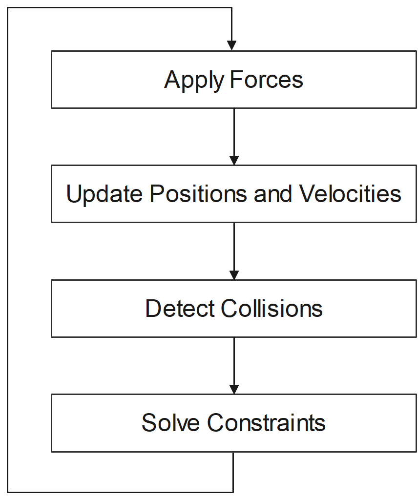
In the following, each of these steps is briefly introduced.
Motion of Rigid Bodies
A rigid body is an object that cannot be deformed. Such objects don’t exist in reality, but they constitute a helpful abstraction that simplifies their simulation. The simulated motion of rigid bodies is based on Newton’s famous Three Laws of Motion:
- First Law (Inertia): If a body is at rest or moving at a constant speed in a straight line, it will remain at rest or keep moving in a straight line at constant speed unless a force acts on it.
- Second Law (Force, Mass, and Acceleration): The acceleration/momentum of a body is proportional in both magnitude and direction to the force imposed on it. For a body whose mass m is constant, this can be written in the form F = ma, where F (force) and a (acceleration) are both vector quantities.
- Third Law (Action and Reaction): When two bodies interact, they apply forces to one another that are equal in magnitude and opposite in direction.
A rigid body possesses has a mass, volume and shape which are constant and a position, orientation and velocity which can change due to forces acting on the it. Positions and orientations are calculated with regards to the body’s centre of mass. The centre of mass of a body is the mean position of the total weight of the body. The body is balanced around the centre of mass.
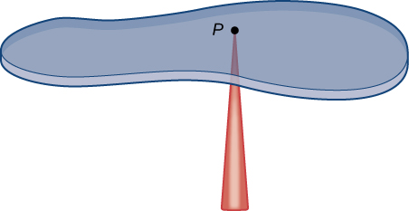
The motion of rigid bodies is typically simulated in three dimensional space. Accordingly, the position of an object can be represented as individual translations along three orthogonal axes. Similarly, the orientation of an object can be represented as individual rotations around the same three orthogonal axes.
The angles with which object rotates around these axes are Euler angles and frequently referred to as yaw, pitch and roll.
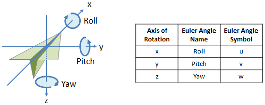
There exist alternative representations for rotations in three dimensional space such as Quaternions. Quaternions represent rotations as four dimensional complex numbers with three components being imaginary. Quaternions are less intuitive to understand as Euler Angles but offer the benefit that they are easier to calculate with and don’t suffer from ambiguous and singular conditions. Bullet Physics employs both rotation representations and converts between them.
Since rigid bodies can change their position and rotation, velocities and forces exist in two varieties. Linear velocity and linear force affect the position of a rigid body. Angular velocity and angular force (frequently named torque) affect the orientation of a rigid body. The inertia of a rigid body with which it resists changes in its position and orientation also exists in two varieties. A regular inertia which resists position changes and a rotational inertia (frequently named moment of inertia) which resists orientation changes.
Collision Detection
Another important aspect of rigid body simulations is the detection of collisions among the bodies and the resolution of these collisions to make the bodies bounce of from each other after collision. The detection of collisions is challenging for two reasons. First, there might be a large number of bodies all of which could potentially collide with each other. Calculating distances between all these bodies is computationally demanding. Second, the bodies themselves might possess complicated shapes which makes it difficult to test if and where these shapes intersect. Dealing with both these aspects at the same time is unfeasible. For this reason, collision detection is separated into the separate steps: a Broad Phase and a Narrow Phase.
Broad Phase
During Broad Phase, every body is tested for intersection with every other body in the simulation. But instead of using the bodies actual shape, an approximation of the shape is created in the form of a bounding volume which can be much easier tested for intersection. Typical approximations are bounding spheres, axis aligned bounding boxes (AABB), oriented bounding boxes (OBB), or convex hulls.
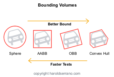
Broad Phase collision detection results in a list of body pairs that might be colliding. If these objects actually collide is subsequently tested during Narrow Phase collision detection.
In the context of Broad Phase collision detection, it’s worthwhile to briefly mention the principle of Space Partitioning. Testing a large number of bodies for collision, even if these bodies possess simple shapes is still a computationally very demanding endeavour, since every body has to be tested for collision with every other body in the simulation. With a naïve approach, a number N of bodies would require a number N^2 of collision tests. These calculations have a run time complexity of O(n2) which means that the computation doesn’t scale well for an increasing number of bodies. Space Partitioning methods serve the purpose of subdividing space and then testing only for collision among those objects that reside within neighbouring subdivisions of space. There exists various Space Partitioning algorithms. Some of the more popular ones are BSP, Octrees, K-D Trees, and R Trees.
Narrow Phase
During Narrow Phase collision detection, pairs of bodies are tested for intersection. This time, the actual shape of the bodies including their orientation is taken into account. For this intersection tests, it makes a fundamental different if the shape of a body is convex or concave.
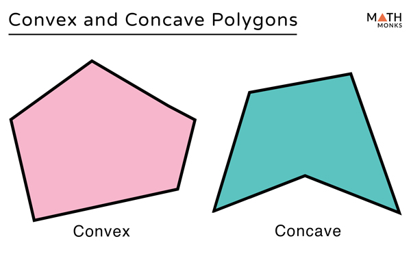
Convex shapes are shapes for which a line that connects any two points within the shape lies entirely within the shape. For Concave objects, this is not the case. Narrow Phase collision detection is based on finding a separating plane between two shapes. If such a plane exists, the shapes don’t intersect. Finding such a plane is much easier for convex objects than for concave objects. For this reason, many Narrow Phase algorithms exist in two versions, a fast version that only supports convex shapes, and a much slower version that also supports concave shapes. Usually, when dealing with concave shapes, the preferred approach is to subdivide a single concave shape into multiple convex shapes and then conduct collision detection on the latter ones.
Solve Constraints
Constraints define restrictions on the motion of rigid objects. Examples of constraints are joints and non-penetration requirements. The former reduce the numbers of freedom with which bodies connected by joints can move with respect to each other. The later prevents bodies from penetrating into each other after a collision.
There are two different approaches for dealing with bodies that violate constraints: force-based and impulse-based. Force-based approaches calculate corrective forces that are applied to the bodies. Impulse-based approaches calculate corrective velocities. In both cases, the corrective values need to be integrated in order to obtain object positions and orientations that no longer violate the constraints (or violate them to a lesser degree). For more information about constraint resolution I refer the reader to the excellent article by Nilson Souto.
The remainder of this article introduces some of the common joints that rigid body dynamics libraries such as Bullet Physics support. The most basic types of constraints are the Hinge, Slider, and Spherical constraint. Without any constraints, a rigid body in a three-dimensional simulation space possesses six degrees of freedom. These are made of three translational degrees of freedom along each axis in the bodies own local coordinate system, and three rotational degrees of freedom around each axis the coordinate system.
Hinge Constraint
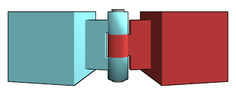
A Hinge Constraint reduces the six degrees of freedom to one, a rotation around a single axis. A typical example of such a joint would be a door hinge.
Slider Constraint
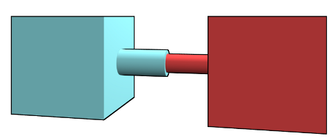
A Slider Constraint reduces the six degrees of freedom to one, a translation along a single axis. A typical example of such a joint would be a piston.
Spherical Constraint
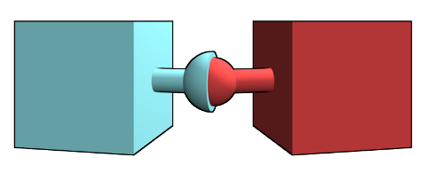
A Spherical Constraint has three degrees of freedom since it only removes the translational degrees of freedom but preserves the rotational ones. A typical example would be a hip joint.
Universal Constraint
The most versatile joints that Bullet Physics provides are universal joints. These are joints in which each of the six degrees of freedom can be constrained individually. Furthermore, each of these individual constraints can either be hard or elastic. Any of the more basic joint types can be imitated by configuring Universal Constraints correspondingly. For this reason, working only with Universal Constraints is usually preferred in Bullet Physics.
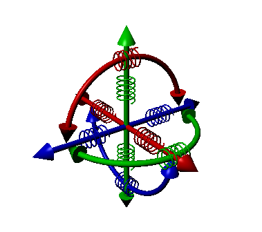
Example Work: Movement Qualities for Non-Anthropomorphic Bodies
In the context of the E2-Create project, Bullet Physics has been employed to create articulated morphologies for non-anthropomorphic bodies that evoke in their movements some of the movement qualities that choreographer Muriel Romero works with.
Movement Qualities
Muriel Romero has developed a creative process that heavily relies on employing
movement qualities as choreographic building blocks. Five of her movement qualities have been selected for simulation in Bullet Physics. The five movement qualities can be described as follows:
- Levitation: Body parts are pulled towards a target position within the dancer’s reach space.
- Fluidity: Body parts move smoothly without taking sharp turns or suddenly changing velocity.
- Particles: Body parts float weightlessly while frequently and erratically changing direction.
- Staccato: Body parts move along straight lines and quickly speed up and slow down at the beginning and ending of a line.
- Thrusting: Body parts propel themselves outwards and rebound afterwards.
Non-Anthropomorphic Articulated Morphologies
Two non-anthropomorphic morphologies were designed using the OnShape
online CAD software. Both morphologies are extremely simple in shape and type of articulation which makes them appear and move in a manner that bears little similarity to a human body. Both morphologies possess a body architecture with a non-branching structure and the joints that connect successive body parts possess one rotational degree of freedom. In both morphologies, the first body part acts as base and fixes the morphology in space. Fixing the base part in space permits to focus solely on movement qualities without having to deal with issues of body balance and locomotion.
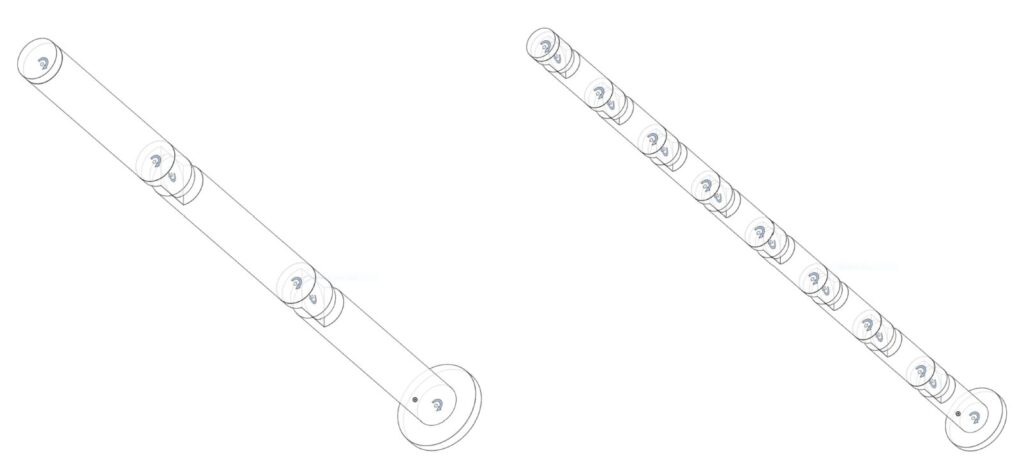
depicted as outlined shapes and rotational joints as curved arrows. The image on the
left shows a morphology that consists of 6 joints and 7 parts. The image on
the right shows a morphology that consists of 17 joints and 18 parts.
Body Behaviours
For the bodies to exhibit autonomous movements, a combination of physical parameter settings and custom designed behaviours was employed. The custom designed behaviours are not directly part of the simulation. Instead, they operate as external routines that cause an articulated morphology to exhibit autonomous movements. They do so either by altering some of the parameters of the body parts or body joints that are assigned to them or by exerting physical forces. Two different behaviours are currently implemented. A behaviour named ForceBehaviour generates forces that impact externally on body parts. A behaviour named RotationBehaviour specifies target angles towards which body joints rotate to. Both behaviours exert their effects either deterministically or randomly. In the latter case, the range of the randomised values and the frequency of their randomisation can be configured. To obtain body movements that exhibit a desired quality, different parameter settings for simulation and behaviours and different body part/joint assignments to behaviours have been explored and evaluated.
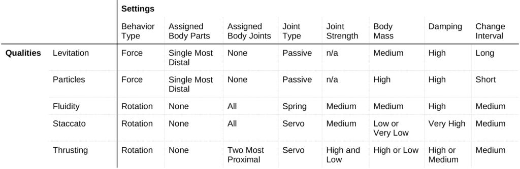
the chosen behaviour, joint and part assignments, joint types, and the most relevant
parameter settings for each of the movement qualities. The terms distal and proximal
refer to the location of a part or joint relative to a morphology’s fixed base.
Dance Performance
The simulated morphologies were integrated into two scenes of a dance performance entitled “Embodied Machine”. In these scenes, the morphologies play the role of artificial dancers that follow their own improvised or choreographed movements. The artificial dancers are present on stage in the form of moving lights. Since the moving lights possess only two rotational degrees of freedom, only a subset of the joints of a simulated morphology could be assigned to a moving light. In the case of the morphology with 6 joints, the first and the last joint were assigned to the pan and tilt axes of a moving light, respectively. In the case of the morphology with 17 joints, each pair of successive joints s is mapped to the pan and tilt axis of a robotic light.
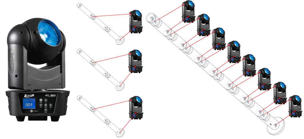
Described here is one of the two performance scenes. In this scene, 16 morphologies with 6 joints each control 16 moving lights. The moving lights are arranged in two circles with 8 lights each. One circle is placed on the stage and the other hanging from a truss. This arrangement has been replicated in the simulation. The moving lights follow their own choreography which progresses through several stages. Initially, one moving light after the other performs the same movement quality (Levitation), then all lights perform the movement quality (Fluidity) in unison. After that, the lights on stage and those hanging perform movement qualities that are in contrast to each other such as Fluidity and Particles or Thrusting and Staccato. Finally, all the lights individually and repeatedly chose a random movement quality.