Summary
The following tutorial introduces the use of a simple generative adversarial network for generating synthetic images. This model can be trained on a collection of images. The model uses a combination of a conventional neural network (ANN) and a convolutional neural network (CNN) to create images.
This tutorial forms part of a series of tutorials on using PyTorch to create and train generative deep learning models. The code for these tutorials is available here.
In this example, the model is trained on images that have been collected on Flickr by using a full text search for the words “dancer, dance, contemporary, solo”.
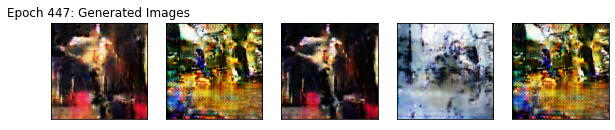
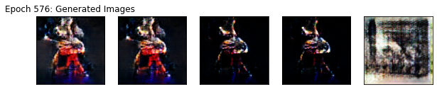
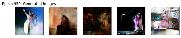
After training the model on about 4000 images for up to 1000 epochs, it generates images such as these.
Imports
The following modules need to be available and imported for this example.
import numpy as np
import torch
import torchvision
from pytorch_model_summary import summary
from torch.utils.data import DataLoader
from torch import nn
from torch import optim
from collections import OrderedDict
import matplotlib.pyplot as plt
import time
import pickle
import math
Compute Device
If a GPU is available for running the model, this device can be selected as follows.
device = 'cuda' if torch.cuda.is_available() else 'cpu'
print('Using {} device'.format(device))
Import Images and Create Dataset
The easiest method to import images that are stored in local directories involves the use of the ImageFolder class that forms part of the torchvision.datasets submodule. This class represents a Dataset for images that can be directly used for creating Dataloaders. This avoids having to write your own code for importing images from directories, converting them into tensors, and implementing a custom Dataset class. The constructor of the ImageFolder class takes two arguments: the top level path to where all images are stored and an instance of the torchvision.transforms.Compose class.
The path provided to the constructor must be one level higher in the directory structure than the directory or directories that contain the images. The reason for this is that the distribution of images across directories is interpreted as classification of the images, where each directory name represents the class label for the images that are contained within it. Since we don’t need class labels for this example, it is fine to store all images in a single directory. Here, this single directory has the name “Flickr_Dancers” and contains approximately 4000 images of dancers and dance settings that have been downloaded from Flickr. The downloaded images have a resolution of 150×150 pixels and contain three colour channels. The Python code used for scraping images from Flickr is described here. The already downloaded images are available here.
The instance of the Compose class which forms part of the torchvision.transforms submodule provides the functionality to process images in the dataset before they are passed as input data into a machine learning model. The constructor of the Compose class takes as argument a list of instances of classes for image processing. Several such classes are provided by the torchvision.transforms submodule. In the code example, only two instances for image processing are passed to the constructor, one for resizing the images and one for converting the images into tensors. Once the Compose class has been instantiated, it will automatically process images in the sequence in which the image processing instances were passed to the constructor.
The code for creating a Dataset for images is as follows:
image_data_path = "../../data/Images"
image_size = 128

transform = torchvision.transforms.Compose([ torchvision.transforms.Resize(image_size), torchvision.transforms.ToTensor() ])

full_dataset = torchvision.datasets.ImageFolder(image_data_path, transform=transform)
This dataset contains all data. The dataset can be split into two datasets, one for training and one for testing, as follows:
test_percentage  = 0.2

dataset_size = len(full_dataset)

test_size = int(test_percentage * dataset_size)
train_size = dataset_size - test_size

train_dataset, test_dataset = torch.utils.data.random_split(full_dataset, [train_size, test_size])
DataLoaders are created from these two datasets as follows:
batch_size = 16

train_dataloader = DataLoader(train_dataset, batch_size=batch_size, shuffle=True)
test_dataloader = DataLoader(test_dataset, batch_size=batch_size, shuffle=False)
Create Models
A generative adversarial network (GAN) consists of two models. One for generating synthetic data from input noise, and the other for discriminating between original data and synthetic data. The former is named “Generator” and the latter “Critique”. A brief introduction to GANs is available here. In this example, the two models operate on images. The Generator model takes as input a tensor containing noise and produces as output a tensor representing synthetic images. The noise vector represents the encoding of the synthetic image. The Critique takes as input a tensor representing images and produces as output a tensor that classifies the images as ether real or fake (synthetic). Both models employ as networks a combination of convolutional neural networks (CNN) and conventional artificial neural networks (ANN).
Create Critique Model
For converting input images into output classes, the Critique model first passes the input images through several convolution layers, then flattens the feature map that is output by the last convolution layer into a one-dimensional feature vector. This feature vector is then passed through several conventional neural network layers with the last layer outputting a single value.
The CNN part of the model successively reduces the size of the feature maps while increasing their number of channels. Each convolution layer is followed by a leaky RelU activation function and a batch normalisation.
The ANN part of the model successively reduces the dimension of the one-dimensional feature vector down to 1. Each ANN layer with the exception of the last one is also followed by a leaky ReLU activation function. The last ANN layer is followed by a Softmax activation function to obtain normalised class probabilities.
The class definition of the Critique model is as follows:
class Critique(nn.Module):
    def __init__(self, image_size, image_channels, conv_channel_counts, conv_kernel_size, dense_layer_sizes):
        super().__init__()

        self.image_size = image_size
        self.image_channels = image_channels
        self.conv_channel_counts = conv_channel_counts
        self.conv_kernel_size = conv_kernel_size
        self.dense_layer_sizes = dense_layer_sizes

        # create convolutional layers
        conv_layers = []

        stride = (self.conv_kernel_size - 1) // 2
        padding = stride

        conv_layers.append(("critique_conv_0", nn.Conv2d(image_channels, self.conv_channel_counts[0], self.conv_kernel_size, stride=stride, padding=padding)))
        conv_layers.append(("critique_lrelu_0", nn.LeakyReLU(0.2)))
        conv_layers.append(("critique_bnorm_0", nn.BatchNorm2d(self.conv_channel_counts[0])))

        conv_layer_count = len(conv_channel_counts)

        for layer_index in range(1, conv_layer_count):
            conv_layers.append(("critique_conv_{}".format(layer_index), nn.Conv2d(self.conv_channel_counts[layer_index-1], self.conv_channel_counts[layer_index], self.conv_kernel_size, stride=stride, padding=padding)))
            conv_layers.append(("critique_lrelu_{}".format(layer_index), nn.LeakyReLU(0.2)))
            conv_layers.append(("critique_bnorm_{}".format(layer_index), nn.BatchNorm2d(self.conv_channel_counts[layer_index])))

        self.conv_layers = nn.Sequential(OrderedDict(conv_layers))
        self.flatten = nn.Flatten(start_dim=1)

        # create dense layers
        dense_layers = []

        last_conv_layer_size = image_size // np.power(2, len(conv_channel_counts))

        #print("last_conv_layer_size ", last_conv_layer_size)

        dense_layer_input_size = conv_channel_counts[-1] * last_conv_layer_size * last_conv_layer_size

        #print("dense_layer_input_size ", dense_layer_input_size)

        dense_layers.append(("critique_dense_0", nn.Linear(dense_layer_input_size, self.dense_layer_sizes[0])))
        dense_layers.append(("critique_dense_lrelu_0", nn.LeakyReLU(0.2)))

        dense_layer_count = len(dense_layer_sizes)
        for layer_index in range(1, dense_layer_count):
            dense_layers.append(("critique_dense_{}".format(layer_index), nn.Linear(self.dense_layer_sizes[layer_index-1], self.dense_layer_sizes[layer_index])))
            dense_layers.append( ( "critique_dense_lrelu_{}".format( layer_index ), nn.LeakyReLU(0.2) ) )

        dense_layers.append( ("encoder_dense_{}".format( len(self.dense_layer_sizes) ), nn.Linear( self.dense_layer_sizes[-1], 1) ) )
        dense_layers.append( ( "encoder_dense_sigmoid_{}".format( len(self.dense_layer_sizes) ), nn.Sigmoid() )  )

        self.dense_layers = nn.Sequential(OrderedDict(dense_layers))

    def forward(self, x):

        #print("x1 s", x.shape)

        x = self.conv_layers(x)

        #print("x2 s", x.shape)

        x = self.flatten(x)

        #print("x3 s", x.shape)

        yhat = self.dense_layers(x)

        #print("yhat s", yhat.shape)

        return yhat
The constructor of the Critique model class takes the following arguments: the size of a square image, the number of image channels, a sequence of channel counts for the convolution layers, the size of the convolution kernels, and a sequence of unit counts for the conventional neural network layers (with the unit count of 1 for the last layer missing, since this layer is added anyway). The model class can be instantiated as follows:
image_size = 128
image_channels = 3
crit_conv_channel_counts = [ 8, 32, 128, 512 ]
crit_conv_kernel_size = 5
crit_dense_layer_sizes = [ 128 ]

critique = Critique(image_size, image_channels, crit_conv_channel_counts, crit_conv_kernel_size, crit_dense_layer_sizes).to(device)
The shapes of the input and output tensors for this model are as follows:
- input tensor: batch_size x image_channels x image_size x image_size
- output tensor: batch_size x 1
Create Generator Model
For generating synthetic images from a one dimensional vector of random values, the Generator model first passes the noise vector through several conventional neural network layers, then un-flattens the output of the last ANN layer into a two dimensional feature map. This feature map is then passed through several deconvolution layers with the last one outputting the synthetic image.
The ANN part of the model successively increases the dimension of the noise vector. Each ANN layer with the exception of the last one is followed by a ReLU activation function.
The CNN part of the model successively increases the size of the feature maps while decreasing the number of channels. Each deconvolution layer with the exception of the last one is preceded by a batch normalisation and followed by a leaky ReLU activation function. The last deconvolution layer is preceded by a batch normalisation and followed by a Sigmoid activation function.
The class definition of the Generator model is as follows:
class Generator(nn.Module):

    def __init__(self, latent_dim, image_size, image_channels, conv_channel_counts, conv_kernel_size, dense_layer_sizes):
        super().__init__()

        self.latent_dim = latent_dim
        self.image_size = image_size
        self.image_channels = image_channels
        self.conv_channel_counts = conv_channel_counts
        self.conv_kernel_size = conv_kernel_size
        self.dense_layer_sizes = dense_layer_sizes

        # create dense layers
        dense_layers = []

        dense_layers.append(("generator_dense_0", nn.Linear(latent_dim, self.dense_layer_sizes[0])))
        dense_layers.append(("generator_relu_0", nn.ReLU()))

        dense_layer_count = len(dense_layer_sizes)
        for layer_index in range(1, dense_layer_count):
            dense_layers.append(("generator_dense_{}".format(layer_index), nn.Linear(self.dense_layer_sizes[layer_index-1], self.dense_layer_sizes[layer_index])))
            dense_layers.append( ( "generator_dense_relu_{}".format(layer_index), nn.ReLU() ) )

        last_conv_layer_size = int(image_size // np.power(2, len(conv_channel_counts)))
        preflattened_size = [conv_channel_counts[0], last_conv_layer_size, last_conv_layer_size]
        dense_layer_output_size = conv_channel_counts[0] * last_conv_layer_size * last_conv_layer_size

        print("preflattened_size ", preflattened_size)

        dense_layers.append( ( "generator_dense_{}".format(len(self.dense_layer_sizes) ), nn.Linear( self.dense_layer_sizes[-1], dense_layer_output_size) ) )

        self.dense_layers = nn.Sequential(OrderedDict(dense_layers))

        self.unflatten = nn.Unflatten(dim=1, unflattened_size=preflattened_size)

        # create convolutional layers
        conv_layers = []

        stride = (self.conv_kernel_size - 1) // 2
        padding = stride
        output_padding = 1

        conv_layer_count = len(conv_channel_counts)
        for layer_index in range(1, conv_layer_count):
            conv_layers.append(("generator_bnorm_{}".format(layer_index), nn.BatchNorm2d(conv_channel_counts[layer_index-1])))
            conv_layers.append(("generator_conv_{}".format(layer_index), nn.ConvTranspose2d(conv_channel_counts[layer_index-1], conv_channel_counts[layer_index], self.conv_kernel_size, stride=stride, padding=padding, output_padding=output_padding)))
            conv_layers.append(("generator_lrelu_{}".format(layer_index), nn.LeakyReLU(0.2)))

        conv_layers.append(("generator_bnorm_{}".format(conv_layer_count), nn.BatchNorm2d(conv_channel_counts[-1])))
        conv_layers.append(("generator_conv_{}".format(conv_layer_count), nn.ConvTranspose2d(conv_channel_counts[-1], self.image_channels, self.conv_kernel_size, stride=stride, padding=padding, output_padding=output_padding)))
        conv_layers.append( ( "generator_sigmoid_{}".format( conv_layer_count), nn.Sigmoid() ) )

        self.conv_layers = nn.Sequential(OrderedDict(conv_layers))

    def forward(self, x):

        #print("x1 s ", x.shape)

        x = self.dense_layers(x)

        #print("x2 s ", x.shape)

        x = self.unflatten(x)

        #print("x3 s ", x.shape)

        yhat = self.conv_layers(x)

        #print("yhat s ", yhat.shape)

        return yhat
The constructor of the Generator model class takes the following arguments: the latent dimension of the image encoding, the size of a square image, the number of image channels, a sequence of channel counts for the deconvolution layers (with the channel count of 3 for the last layer missing, since this layer is added anyway), the size of the deconvolution kernels, and a sequence of unit counts for the conventional neural network layers. The model class can be instantiated as follows:
latent_dim = 64
image_size = 128
gen_conv_channel_counts = [ 512, 128, 32, 8 ]
gen_conv_kernel_size = 5
gen_dense_layer_sizes = [ 128 ]

generator = Generator(latent_dim, image_size, image_channels, gen_conv_channel_counts, gen_conv_kernel_size, gen_dense_layer_sizes).to(device)
The shapes of the input and output tensors for this model are as follows:
- input tensor: batch_size x latent_dim
- output tensor: batch_size x image_channels x image_size x image_size
Optimisers and Loss Functions
To update the weights of the two models during training, two individual Adam optimisers are used. In this example, both optimisers use the same learning rate. These optimisers are instantiated as follows:
gen_learning_rate = 1e-4
crit_learning_rate = 1e-4

critique_optimizer = torch.optim.Adam(critique.parameters(), lr=crit_learning_rate)
generator_optimizer = torch.optim.Adam(generator.parameters(), lr=gen_learning_rate)
Two different loss functions are used, one for the Critique model and one for the Generator model. The loss functions internally use binary cross-entropy loss to quantify the classification error of the Critique model.
bce_loss = nn.BCELoss()The loss function for the Critique model is named “crit_loss”. It calculates two individual losses with are then scaled and summed to obtain a single loss. The first loss is based on the difference between the Critique’s classification of “real” images (the ones that are in the dataset) and a vector containing values of 1. The second loss is based on the difference between the Critique’s classification of “fake” images (the ones output by the Generator model) and a vector containing values of 0. If the Critique makes no mistakes, then it would produce for the classification of “real” images a vector containing values of 1 and for the classification of “fake” images a vector containing values of 0. The binary cross entropy loss between these vectors drive the training of the Critique.
The definition of the “crit_loss” is as follows:
# crictique loss function
def crit_loss(crit_real_output, crit_fake_output):
    _real_loss = bce_loss(crit_real_output, torch.ones_like(crit_real_output).to(device))
    _fake_loss = bce_loss(crit_fake_output, torch.zeros_like(crit_fake_output).to(device))

    _loss = (_real_loss + _fake_loss) * 0.5
    return _loss
The loss function for the Generator model is named “gen_loss”. It calculates a single loss. This loss is based on the difference between the Critique’s classification of “fake” images and a vector containing values of 1. The Generator is successful if the synthetic images it generates are classified as real by the Critique. In this case, the Critique produces a vector containing values of 1. The binary cross entropy loss between these vectors drive the training of the Generator.
The definition of the “gen_loss” is as follows:
def gen_loss(crit_fake_output):
    _loss = bce_loss(crit_fake_output, torch.ones_like(crit_fake_output).to(device))
    return _loss
Training and Testing Functions
A total of four different functions are defined for conducting training and testing steps: a training and a testing step function for the Critique model and a training and testing step function for the Generator model. The functions for the Critique model are named “crit_train_step” and “crit_test_step” and take as input two tensors, one representing a batch of real images, the other a batch of noise vectors. The functions for the Generator model are named “gen_train_step” and “gen_test_step” and take as input one tensor representing a batch of noise vectors. All these functions compute and return loss values. The functions used for training also calculate the gradients of the loss functions and update the trainable parameters of the Critique and Generator model, respectively. The functions used for testing suppresse gradient calculation and leave the trainable model parameters unchanged.
def crit_train_step(real_images, random_encodings):

    critique_optimizer.zero_grad()

    with torch.no_grad():
        fake_output = generator(random_encodings)
    real_output = real_images

    crit_real_output =  critique(real_output)
    crit_fake_output =  critique(fake_output)

    _crit_loss = crit_loss(crit_real_output, crit_fake_output)

    _crit_loss.backward()
    critique_optimizer.step()

    return _crit_loss

def crit_test_step(real_images, random_encodings):
    with torch.no_grad():
        fake_output = generator(random_encodings)
        real_output = real_images

        crit_real_output =  critique(real_output)
        crit_fake_output =  critique(fake_output)

        _crit_loss = crit_loss(crit_real_output, crit_fake_output)

    return _crit_loss

def gen_train_step(random_encodings):

    generator_optimizer.zero_grad()

    generated_images = generator(random_encodings)

    crit_fake_output = critique(generated_images)

    _gen_loss = gen_loss(crit_fake_output)

    _gen_loss.backward()
    generator_optimizer.step()

    return _gen_loss

def gen_test_step(random_encodings):
    with torch.no_grad():
        generated_images = generator(random_encodings)

        crit_fake_output = critique(generated_images)

        _gen_loss = gen_loss(crit_fake_output)

    return _gen_loss
The function named “train” performs the actual training of the two models by calling the train and test step functions repeatedly. This function takes as arguments the train and test Dataloaders and the number of epochs. It then runs through an outer loop and two inner loops. The outer loop iterates over all epochs. The first inner loop iterates over all the batches provided by the train Dataloader, The second inner loop iterates over all the batches provided by the test Dataloader. In each of these inner loops, the loss returned by the loss functions are added to a dictionary. This dictionary contains the history of the training process. The training function is defined as follows:
def train(train_dataloader, test_dataloader, epochs):

    loss_history = {}
    loss_history["gen train"] = []
    loss_history["gen test"] = []
    loss_history["crit train"] = []
    loss_history["crit test"] = []

    for epoch in range(epochs):

        start = time.time()

        crit_train_loss_per_epoch = []
        gen_train_loss_per_epoch = []

        for train_batch, _ in train_dataloader:
            train_batch = train_batch.to(device)

            random_encodings = torch.randn((train_batch.shape[0], latent_dim)).to(device)

            # start with critique training
            _crit_train_loss = crit_train_step(train_batch, random_encodings)

            _crit_train_loss = _crit_train_loss.detach().cpu().numpy()

            crit_train_loss_per_epoch.append(_crit_train_loss)

            # now train the generator
            for iter in range(2):
                _gen_loss = gen_train_step(random_encodings)

                _gen_loss = _gen_loss.detach().cpu().numpy()

                gen_train_loss_per_epoch.append(_gen_loss)

        crit_train_loss_per_epoch = np.mean(np.array(crit_train_loss_per_epoch))
        gen_train_loss_per_epoch = np.mean(np.array(gen_train_loss_per_epoch))

        crit_test_loss_per_epoch = []
        gen_test_loss_per_epoch = []

        for test_batch, _ in test_dataloader:
            test_batch = test_batch.to(device)

            random_encodings = torch.randn((train_batch.shape[0], latent_dim)).to(device)

            # start with critique testing
            _crit_test_loss = crit_test_step(train_batch, random_encodings)

            _crit_test_loss = _crit_test_loss.detach().cpu().numpy()

            crit_test_loss_per_epoch.append(_crit_test_loss)

            # now test the generator
            _gen_loss = gen_test_step(random_encodings)

            _gen_loss = _gen_loss.detach().cpu().numpy()

            gen_test_loss_per_epoch.append(_gen_loss)

        crit_test_loss_per_epoch = np.mean(np.array(crit_test_loss_per_epoch))
        gen_test_loss_per_epoch = np.mean(np.array(gen_test_loss_per_epoch))

        if epoch % weight_save_interval == 0 and save_weights == True:
            torch.save(critique.state_dict(), "results/weights/critique_weights_epoch_{}".format(epoch))
            torch.save(generator.state_dict(), "results/weights/generator_weights_epoch_{}".format(epoch))

        plot_gan_outputs(generator, epoch, n=5)


        loss_history["gen train"].append(gen_train_loss_per_epoch)
        loss_history["gen test"].append(gen_test_loss_per_epoch)
        loss_history["crit train"].append(crit_train_loss_per_epoch)
        loss_history["crit test"].append(crit_test_loss_per_epoch)

        print ('epoch {} : gen train: {:01.4f} gen test: {:01.4f} crit train {:01.4f} crit test {:01.4f} time {:01.2f}'.format(epoch + 1, gen_train_loss_per_epoch, gen_test_loss_per_epoch, crit_train_loss_per_epoch, crit_test_loss_per_epoch, time.time()-start))

    return loss_history
To visually verify the progress of the training, the training function calls after each epoch a function named “plot_gan_outputs”. This function draws an image in which several synthetic images generated by the Generator are placed in a row. This function takes as arguments the Generator model, the current epoch, and the number of images that the Generator should generate. This function is defined as follows.
def plot_gan_outputs(generator, epoch, n=5):

    generator.eval()

    plt.figure(figsize=(10,4.5))
    for i in range(n):
      ax = plt.subplot(1,n,i+1)

      generator.eval()
      with torch.no_grad():
         random_encoding = torch.randn((1, latent_dim)).to(device)
         gen_img  = generator(random_encoding)
      generator.train()

      gen_img = gen_img.cpu().squeeze().numpy()
      gen_img = np.clip(gen_img, 0.0, 1.0)
      gen_img = np.moveaxis(gen_img, 0, 2)

      plt.imshow(gen_img)
      ax.get_xaxis().set_visible(False)
      ax.get_yaxis().set_visible(False)
      if i == 0:
          ax.set_title("Epoch {}: Generated Images".format(epoch))
    plt.show()

    generator.train()
The “train” function can be called as follows:
epochs = 1000

loss_history = train(train_dataloader, test_dataloader, epochs)