Machine Learning is a subfield of Artificial Intelligence. Artificial Intelligence is a synthetic natural science that studies natural forms of intelligence by building models that exhibit aspects of intelligence. Such aspects include capabilities such as: coordinate body movements, perceive the environment, learn from experience, plan actions, etc. Machine Learning deals with learning from experience.
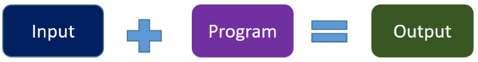
Automated Programming
From a computer science point of view, Machine Learning is a programming approach in which the algorithms that process data are not manually implemented but instead generated automatically based on the data. Therefore, instead of spending time on devising an algorithms for data processing, a computer scientist focuses predominantly on the data. As rule of thumb, better data leads to better automatically generated algorithms.

The main benefit of Machine Learning over conventional programming is that Machine Learning can come up with algorithms for data processing that would be extremely difficult to discover manually. The main drawback of Machine Learning is that most of the time, the exact functioning of the automatically created algorithm is incomprehensible. Accordingly, debugging or modifying such algorithms can be very difficult.
Types of Machine Learning
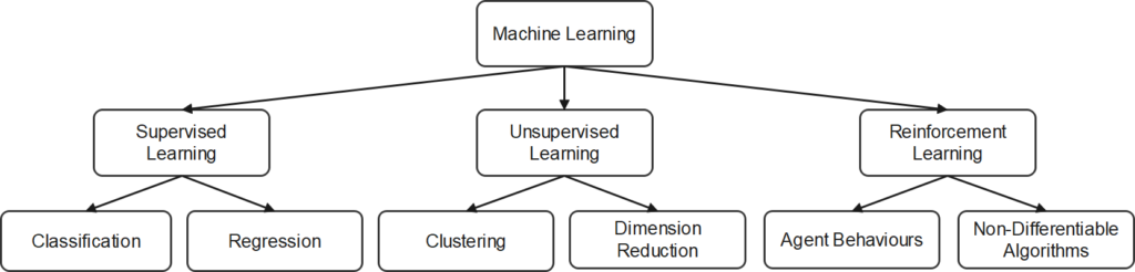
There exists a small number of basic types of Machine Learning. These types are independent from the specifics of an actual implementation. The different types are: Supervised Learning, Unsupervised Learning, and Reinforcement Learning. Supervised learning deals with the learning of mathematical correspondences between input data and output data buy providing examples of input and output data. Unsupervised learning deals with finding statistical patterns in data without providing correct examples of input and output correspondences. Reinforcement Learning is a form of trial and error learning which operates with rewards and punishments. Some of the Machine Learning types exist in different varieties. Supervised Learning can be divided into two subtypes, which are Classification and Regression. Classification deals with categorising data and assigning discrete labels to categories. Regression deals with finding continuous relationships between input and output data. Unsupervised Learning can also be subdivided into two subtypes: Clustering and Dimension Reduction. Clustering deals with organising data into groups based on similarity criteria. Dimension Reduction deals with mapping data from a high dimensional into a low dimensional space while preserving the main distinguishing characteristics of the data. Reinforcement Learning could also be divided into two subtypes which I have named here Agent Behaviours and Non-Differentiable Algorithms. Agent Behaviours refer to what is commonly done with Reinforcement Learning: an Agent learns to interact with an environment in such a manner that it receives a maximum reward for its actions. The principle of trial and error learning and agent environment interaction can be rephrased for dealing with algorithms that cannot be mathematically specified. Such algorithms can be learned through reinforcement learning.
In the remainder of this article, several algorithms will be briefly introduced for the following types of machine learning: Classification, Regression, and Clustering. Algorithms for Reinforcement Learning are discussed in a different article. For readers interested in algorithms for dimensionality reduction, I good starting point are these two articles:
- Top 10 Dimensionality Reduction Techniques For Machine Learning
- 11 Dimensionality reduction techniques you should know in 2021
Machine Learning Algorithms
A further distinction between Machine Learning methods can be made based on the type of algorithms they employ. An algorithm typically takes the form of mathematical equations that possess a more or less large number of parameters that can be configured. The learning part in Machine Learning consists of the automated configuration of these parameters. Other than that, the algorithms themselves are not changed in this process (unlike for example in Evolutionary Programming). An algorithm whose parameters has been configured through Machine Learning is named a model. This model can then be used to make predictions based on new input data that has not been used during learning.
In the following, several different classical machine learning models are briefly surveyed. These algorithms are called classical to differentiate them from the new breed of algorithms that are used in Deep Learning. Compared to Deep Learning, classical algorithms possess much fewer parameters and can therefore be trained faster. But because of the small number of parameters, classical algorithm are not very flexible and usually cannot deal with unstructured and high dimensional data such as raw images or raw audio.
Algorithms for Classification
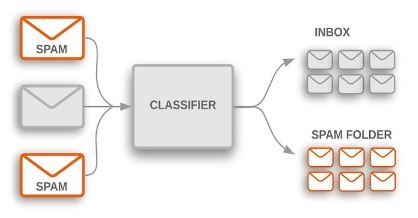
The goal of classification is to group data into several classes by assigning discrete labels to them. The simplest form of classification deals with only two categories. This is called a binary classifier. A typical example for this is an email spam filter that classifies emails as either belonging to the class “Spam” or the class “Non-Spam”.
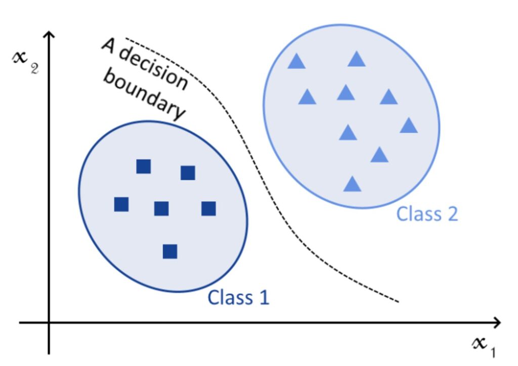
The decision whether a particular instance of data (such as an email) belongs to one class or another (such as Spam or Non-Spam) is akin to drawing a boundary between the two classes and then testing on which side of a boundary the instance lies.
The Binary Classification Approach can be extended to Multiclass Classification by conducting pairwise binary classifications between all classes. The two basic strategies for doing this are One-Versus-Rest and One-Versus-One. In both cases, an Instance is classified through multiple Binary Classifications. In One-Versus-Rest, each of these Binary Classifications classifies an instance as belonging or not belonging to each category in turn. In One-Versus-One, each Binary Classification classifies an instance for each pairwise combination of classes. This approach requires a much higher number of Binary Classification steps than One-Versus-Rest.
Algorithm for Classification – Decision Tree
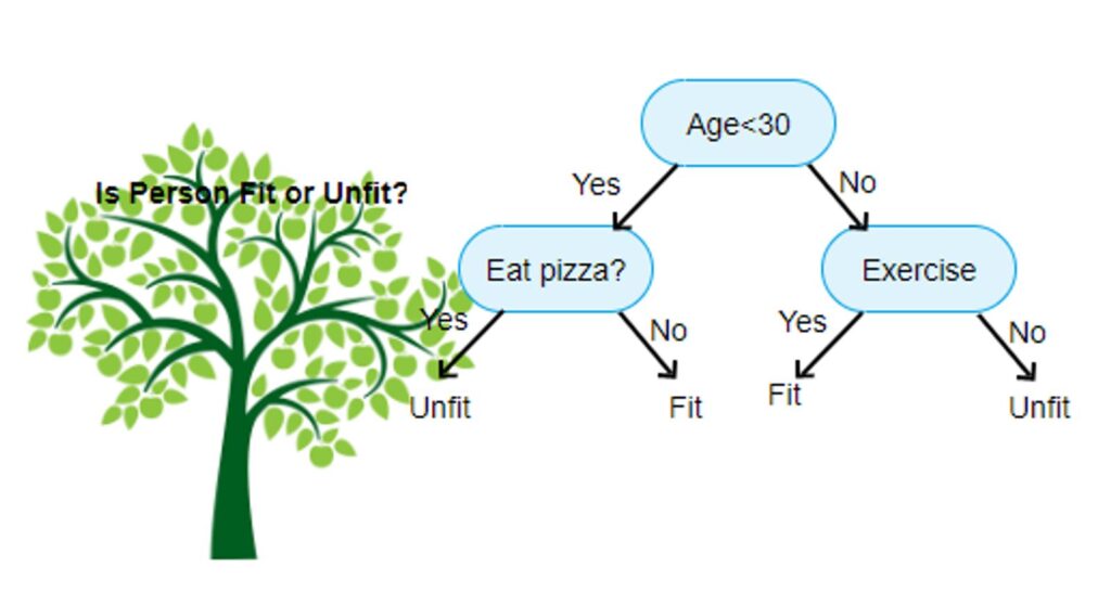
A Decision Tree is a fairly old classification algorithm that takes the form of a binary tree in which each fork in the tree asks a yes-or-no question. The leaves of the tree represent the class labels. Input data enters the tree at its root and then zig-zags through the tree’s branches depending on whether the questions that are asked about the data are replied to with yes or no. A single decision tree is not a very powerful classifier and is therefore frequently used in combination with other decision trees. Such a combination of multiple decision trees is called a Random Forest Classifier.
Algorithm for Classification – Support Vector Machine
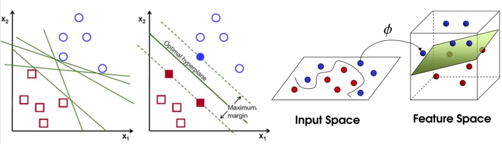
A Support Vector Machine creates linear decision boundaries between classes. In higher dimensions, such a linear decision boundary is a hyperplane. The name of this algorithm stems from the fact that it specifies the surface normal to the hyperplane as support vector. The algorithm places the hyperplane in such a way that the distance between the plane and data instances of different classes is maximally large. This makes this algorithm fairly robust since it prevents misclassifications of data instances that are only minimally different from those it has been trained on. A unique property of Support Vector Machines is that they can separate classes through which no hyperplane that possesses the same dimension as the data fits by moving into a higher dimension.
Algorithm for Classification – Naïve Bayes
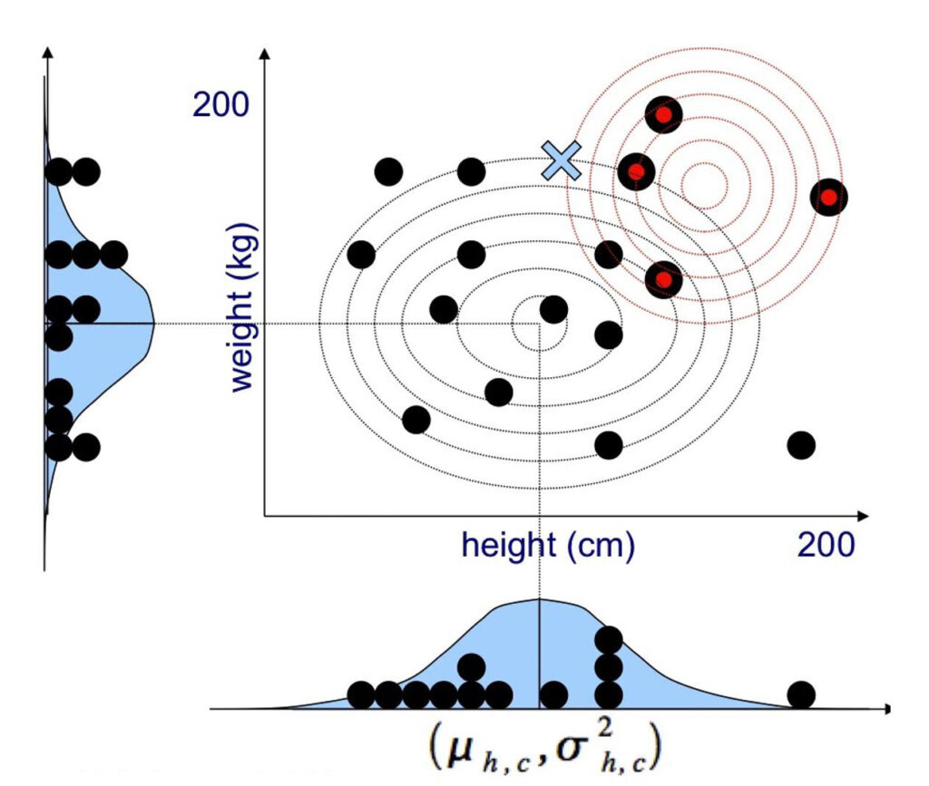
A Naïve Bayes Classifier is a probabilistic method that is based on Bayes Theorem.
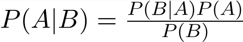
Using Bayes theorem, we can find the probability of an event A happening, given that an event B has occurred. This can be translated into a classification problem by stating that event A represents a class and event B represents a data instance.
A Naïve Bayes classifier is named naïve because it assumes that all data features contribute independently to whether a data instance belongs to a certain class or not. The probability distribution of a class is frequently modelled as a multi-variate Gaussian in which each variable corresponds to one feature of the data. Naïve Bayes Classifiers are fast and easy to implement but their biggest disadvantage is the requirement that data features are independent of each other.
Algorithms for Regression
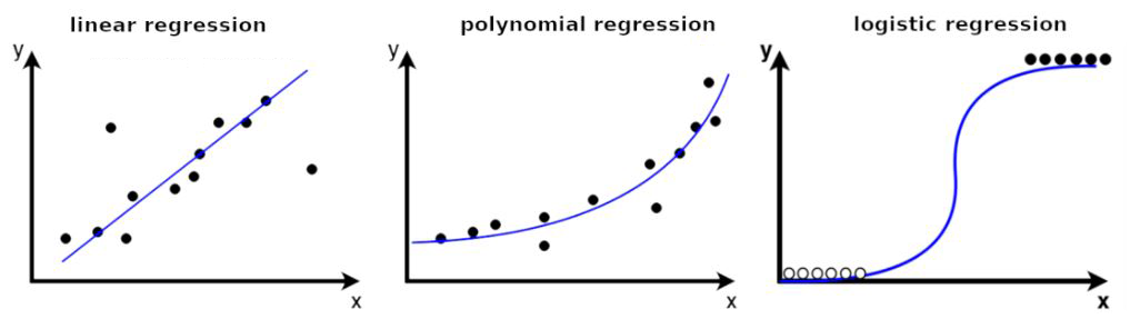
Regression models a continuous relationship between dependent and independent variables. It does so by approximating the true relationship between the variables with a mathematical function. In principle, any type of mathematical function can be used for this purpose as it is differentiable. Nevertheless, only a handful of functions have become popular for this task: linear functions, polynomial functions, and logistic functions. The corresponding types of regression are named linear regression, polynomial regression, and logistic regression.
Since linear functions are a special case of polynomial functions, they will be explained together.
Algorithm for Regression – Polynomial Regression

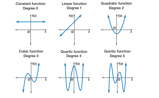
A polynomial function consists of an additive series of integer powers of the independent variable each multiplied with its own coefficient. The highest integer power represents the degree of a polynomial function. A polynomial function with degree 1 is identical with the linear function. Polynomial functions of higher degree can represent more complicated functional relationships between dependent and independent variables.
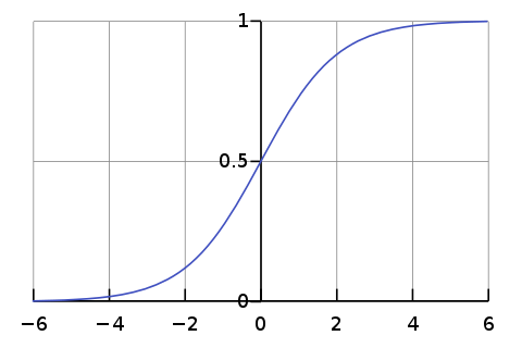
Algorithm for Regression – Logistic Functions
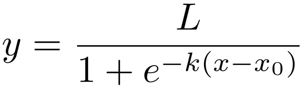
Logistic regression works well in cases where the values of the dependent variable cluster in two groups with values within the same group being very similar to each other. This resembles a classification problem. Accordingly, logistic regression can be used for classification.
Algorithms for Clustering
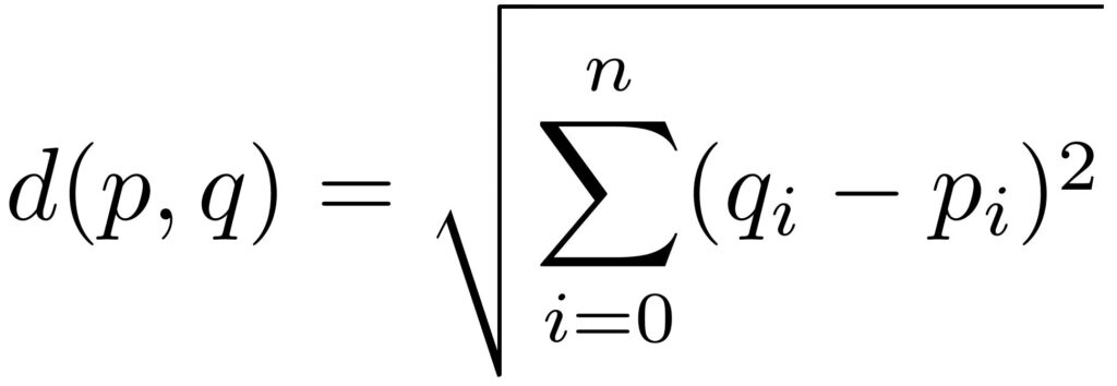
Clustering assigns data instances to groups (clusters). Contrary to classification, no examples are given to the algorithm what these clusters are and which data instances belong to which cluster. What needs to be specified though are criteria for assessing how similar data instances are with respect to each other. Very frequently, the similarity measure is based on the Euclidean distance between the feature values of the data instances.
Algorithms for Clustering – K-Means
For the K-Means clustering algorithm, the number of clusters needs to be known in advance. The algorithm starts by specifying random positions for each cluster centroid. It then iterates as follows: each data instance is assigned to the cluster to whose centroid it is closest, then the centroid of each cluster is updated by setting it to the average of all data instances it contains. These two steps repeat until the centroids no longer change.
Algorithms for Clustering – Mean-Shift
For the Mean-Shift clustering algorithm, the number of clusters does not need to be known in advance and is determined by the algorithm. The algorithm starts with a large number of clusters whose centroids are distributed covering the entire data domain. It then iterates as follows: data instances that are below a given distance from a cluster’s centroid are assigned to this cluster, then the centroid of each cluster is set to the average of all data instances it contains, then clusters whose centroids are very close to each other are fused into a single cluster. The algorithm ends when the number of clusters and their centroids no longer change.
Algorithms for Clustering – DBSCAN
For the DBSCAN clustering algorithm, the number of clusters does not need to be known in advance and is determined by the algorithm. The algorithm starts with zero clusters. In the iterates as follows: an arbitrary data instance that doesn’t yet belong to a cluster is assigned to a new cluster whose centroid lies at the position of the data instance. If there are at least a minimum number of data instances within a maximum radius, these data instances are also assigned to the cluster. Additional data instances keep being assigned to the cluster until the previous condition is no longer fulfilled. The iteration ends if less than a minimum number of data instances can be assigned to a cluster.
Animation of the DPSCAN Clustering Algorithm Gradually Locating Three Clusters.
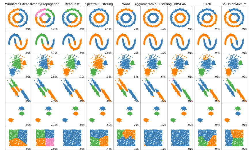
The Python Machine-Learning library Scikit Learn implements all these clustering algorithms as well as several more. The documentation of this library provides a useful overview of how different clustering algorithms handle different data distributions.
Bias and Variance / Underfitting and Overfitting
Before concluding this article, it is useful to introduce a core concept and dilemma of Machine-Learning. The principle of this dilemma can be easily exemplified with polynomial regression. To terms are at centre of this dilemma: Bias and Variance.
Bias is the difference between the predictions of a model and the correct values. Models that are based on simple algorithms with only a few trainable parameters produce high errors in their prediction. These models are said to have a high bias. Another term that is used in this context is Underfitting. These models are said to underfit the data.
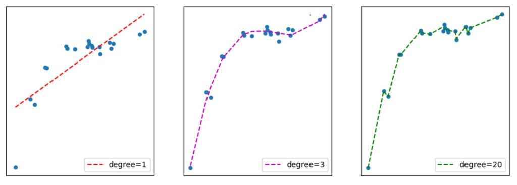
Variance refers to the variability of the predictions a model can make. Models that are based on more sophisticated algorithms with many trainable parameters produce predictions that match the correct values of the data instances that have been used for training very well. At the same time, such models have become overly sensitive to these data instances and might also predict the outliers. For this reason, such models can perform very badly when predicting data that has not been used for training. Another term that is used in this context is Overfitting. These models are said to overfit the data.
The following three graphs illustrate the principle of Bias and Variance in the case of polynomial regression .
Training and Test Set
The use of data for training is another topic that is relevant for any form of Machine Learning and that is also related to the Bias / Variance issue. Training data contains instances of data that are considered representative of the likely infinite number of examples that exist in the data domain. Using all these instances for training a Machine Learning model and then evaluating the model with very same data is a bad idea. The reason for this should be evident from the Bias / Variance issue. By choosing a model with very high variance, we can be certain that the model will learn to predict all training data instances with high accuracy. But we cannot be certain that the model will also do so for data instances that is hasn’t encountered during training. But it is these new data instances that are the most relevant ones when we deploy the model to solve real world problems. Therefore, it is crucial that we can already assess during training if a model is likely going to perform well on data that is not used for training. Only if that is the case, then the model is able to apply what it has learned to general real world data. In that case, it is said that the model generalises well.
Accordingly, it is considered good practice to not train a model on an entire dataset but only parts of it. This part is named Training Set. The remainder and typically much smaller part of the dataset is then used for testing purposes. This part is named Test Set. In some cases, the division of the dataset also includes was is named a Validation Set. In this case, model training is still done using the Training Set. But the continuous testing of the training progress is done with the Validation Set instead of the Test Set. The Test Set is then only used for the final evaluation of the model. In most cases, splitting a dataset into Training and Test Set is considered sufficient. The percentages chosen for Training and Test Set depend on the size of the data set. Typically, for small datasets with “only” a few thousand examples, approximately 90% of the dataset goes into the Training Set and 10% into the Test Set. If the dataset is much larger (millions or more example), then something like 98% go into the Training Set and 2% into the Test Set. But these percentages are just first assumptions and some experimentation is usually required.