Artificial Neural Networks (ANN) are a category of Machine Learning algorithms that are inspired by how biological neurons in a brain organise into networks and process data. While ANNs form the basis for state of the art deep learning models, their original invention dates quite far back. In 1957, Franck Rosenblatt developed the concept of the Perceptron at the Cornell Aeronautical Laboratory. The Perceptron mimics on a very abstract level the operation of a single biological neuron.
Biological Neurons
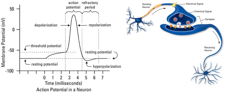
In a nutshell, a biological neuron consists of a main cell body named Soma, multiple cell branches named Dendrites, and one extended cell branch named Axon. Such a neuron transmits information in the form of electrical signals that arrive through Dendrites in the Soma and that are (or are not) propagated along the Axon. The “decision” of a neuron whether to propagate an electrical signal constitutes the neuron’s “computational” capability. Electrical signals are represented as voltage differences across the cell membrane. This so called membrane potential assumes only discrete values. The strength of an electrical signal is therefore not encoded in its magnitude but in the frequency with which discrete spikes in the membrane potential arrive at the Soma. The electrical signal is only propagated along the Axon if the signal strength exceeds a certain threshold.
Perceptron
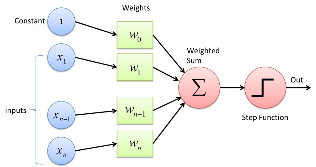
A Perceptron abstracts the operation of a biological neuron in several ways. Electrical signals are represented as numerical values. A Perceptron disposes with the frequency encoding of signal strength. Instead, the magnitude of a numerical value encodes the strength of a signal. The amount of attenuation a signal experiences when passing from the Axon of one neuron to a Dendrite of another neuron is represented by a weighting factor. The combination of all electrical signals in the Soma is represented as a summation. The threshold above which a neuron propagates a signal is represented as a combination of a bias value and a step function.
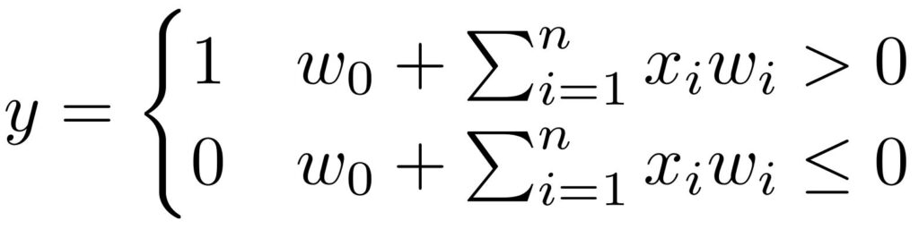
Accordingly, a Perceptron conducts the following computations. It multiplies each component of a multidimensional input signal by a weighting factor. The scaled input signals are then summed together with the bias value. This sum is then passed through a step function with outputs zero if the sum is smaller than or equal to zero and one otherwise.
The Perceptron and with it artificial neural networks fell out of favour because of serious limitations in their functionality. For instance, a Perceptron is not able to solve the XOR problem. Artificial neuronal networks only returned to scientific interest after several improvements have been made. The most important improvements include: multiple artificial neurons are combined with each other, additional functions for processing the summed input signal are introduced, the prediction error of neurons that are not directly generating the final output can be calculated, and more sophisticated update rules for changing the parameters of an artificial neural network have been developed. With these improvements, neural networks have now become an almost de-facto implementation standard for any Machine Learning task including classification, regression, clustering, dimensionality reduction, and reinforcement learning.
Multilayer Networks
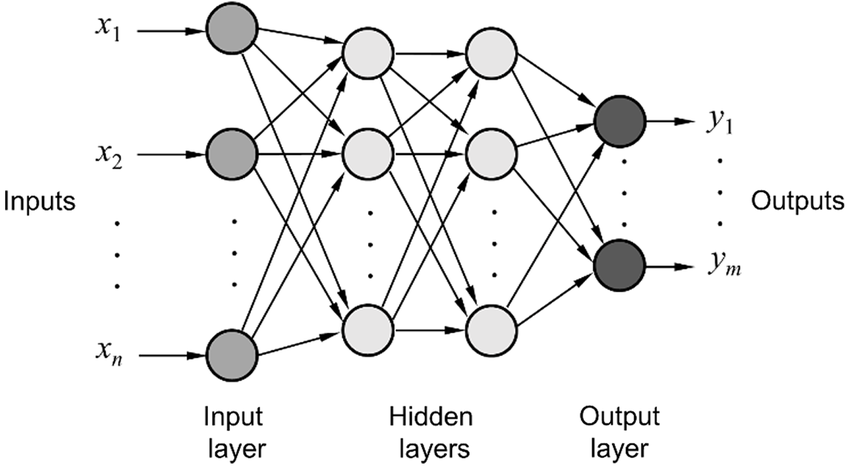
A neural network can consist of more than only one artificial neuron. In a network, neurons can receive input signals from other neurons and they can pass their output signals to other neurons. In neural networks, artificial neurons are frequently organised in layers. A neural network typically consists of at least two layers. A first layer named Input Layer which receives as input directly the features of data instances. For this reason, the number of neurons in the Input Layer equals the number of features in the input data. A last layer named Output Layer which outputs the prediction of the neural network. These can be class probabilities in a classification task or numerical values in a regression task. Accordingly, the number of neurons in the Output Layer is given by the numbers of features of the prediction. Between the Input and Output Layers can be an arbitrary number of additional layers. These internal layers are called Hidden Layers. Neurons in Hidden Layers receive input signals from neurons in previous layers and pass their output signals on to neurons in subsequent layers. The number of Hidden Layers and the number of neurons in a Hidden Layer is not pre-specified by the number of features in the input and output data. This makes their choice somewhat of a mystery. Typically, these numbers can only be found through an empirical approach. As a rule of thumb, if a network significantly underfits the data, the number of Hidden Layers and neurons per layer should be increased. If the opposite is the case and the network significantly overfits the data, then the number of Hidden Layers and neurons per layer should be decreased. And additional rule of thumb: increasing the number of Hidden Layers has a bigger impact on improving the computational capabilities of a network than increasing the number of neurons in a Hidden Layer.
Activation Functions
The step function used in the Perceptron is an example of an activation function. The purpose of an activation function is to introduce a non-linearity in the processing of signals. Without such a non-linearity, an artificial neural network could only learn to approximate linear functional relationships between input and output data. It is thanks to non-linear activation functions, that neural networks can in principle approximate any mathematical function. A large number of different activation functions have been introduced over time, but only a handful of them is commonly used nowadays. These activation functions are: identity, rectilinear unit (ReLU), logistic, hyperbolic tangent (tanh), leaky rectilinear unit (Leaky ReLU), and exponential linear unit (ELU).
Plots of the activation functions look as follows:
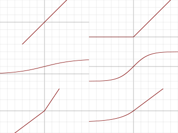
The equations for the activation functions are as follows:
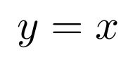
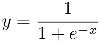
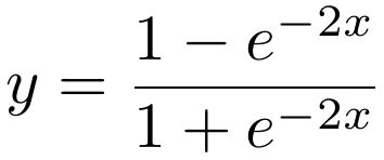
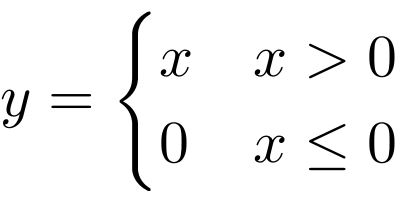
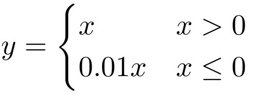

Choosing the most appropriate activation function is not always easy. Some rules of thumb are: The identity activation function is used for neurons in the output layer if the network is used for regression. The logistic activation function is used for neurons in the output layer if the network is used for classification. The tanh activation function is used for hidden neurons in recurrent neural networks. The rectified linear unit ReLU is used for hidden neurons in all other neural networks. The Leaky ReLU or ELU activation function is used to prevent “dead” neurons. These are neurons that always have zero activity.
Loss Functions
Loss functions are used to quantify the prediction mistake that a neural network makes. Loss functions form the basis for training a neural network and for assessing its performance. There exists a large number of different loss functions, but all of them fall into one of two principal categories. Deterministic loss functions return a scalar error value based on the difference between correct and predicted output values. Probabilistic loss functions return a scalar error value based on the probability that a correct output value can be drawn from a predicted probability distribution. Additional loss functions can be employed to evaluate domain specific aspects of the predicted values, for example whether the vector of all output features has unit length. These additional loss functions are usually used in combination with the more universal loss functions that are described below.
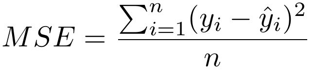
Mean Square Error
Mean square error (MSE) measures the average of the squared difference between correct and predicted values. Due to squaring, predictions which are far away from the correct values are penalized heavily in comparison to predictions the deviate less. Mean Square Error is commonly used for regression tasks.
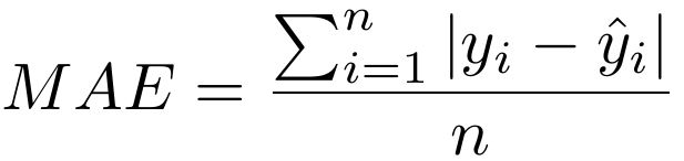
Mean Absolute Error
Mean absolute error (MAE) measures the average of the sum of absolute differences between correct and predicted values. MAE is more robust than MSE to outliers since it doesn’t square the differences. Mean Absolute Error is less commonly used for regression tasks.
Cross-Entropy
Cross-entropy loss is commonly used for classification tasks. Cross-entropy loss increases as the predicted probability diverges from the actual class label. Cross entropy loss penalizes heavily the predictions that are confident but wrong.

Back Propagation
When a neural network receives at its input layer data and produces at its output layer the predictions, it operates in a forward manner, i.e. data travels from input layer to output layer. This is called Forward Propagation. The operation in the opposite direction is called Back Propagation (BP) and plays an important role during training. Training involves the tuning of the parameters of the neural network with the goal of reducing the error that the network makes. The parameters that are modified during training are the weights and bias of each neuron.
Back Propagation consists of two steps. In a first step, Back Propagation evaluates the error that each neuron contributes to the overall prediction. In a second step, the derivative of the error is calculated with respect to the parameters of the neurons. These derivates correspond to gradients that are later used to update the parameters of the neuron using an optimisation algorithm such as Gradient Decent.
The error that each neurons at the output layer produces is quantified by the cost function. The cost function is simply the averaged loss over all training examples. Determining the error of each neuron at the output layer is straight forward, since this is exactly what the cost-function returns. For neurons that are in hidden layers, attributing their contribution to the error is more difficult. Back Propagation calculates the error in neurons in previous layers recursively. This is done by taking a weighted sum of all the errors from the nodes in the layer to which the nodes in the previous layer send their signals to.
The changes that need to be made to the parameters of each neuron to minimise its contribution to the network’s error are determined by calculating the derivative of this error with respect to the neuron’s parameters (weights and bias). Since the error results from a sequence of multiple mathematical operations (activation, weighted summation), the calculation of the derivatives requires the use of the chain rule. This article doesn’t go into the details concerning the math involved in Back Propagation. Readers who are interested in this topic can for instance look at one of the following to articles:
Gradient Descent
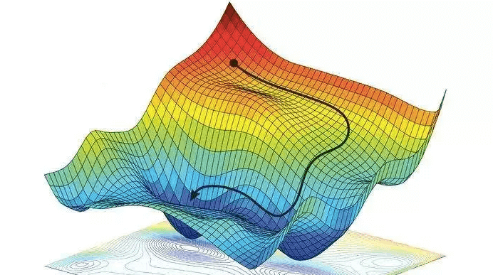
Gradient Descent is the method employed by an optimisation algorithm to find the minimum in an error function. It does so by following the gradient of the error function which has previously been calculated using Back Propagation. Gradient Descent can be visualised as a traversal through a mountainous territory (the error landscape) with peaks representing high error values and valleys representing low error values. The goal of Gradient Descent is to traverse to territory until the lowest point (the global minimum) is found.
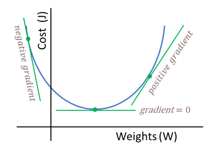
Traversal of the error landscape is done by updating at each iteration of Gradient Descent the network parameters by adding the scaled values of the gradient.
new parameters = old parameters + gradient * alpha
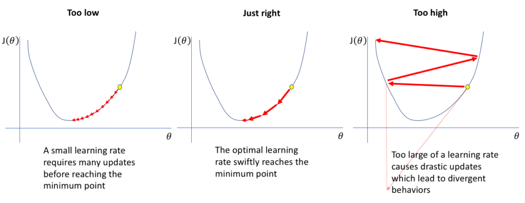
Alpha is referred to as learning rate. Choosing a good learning rate can be tricky. If the learning rate is too small, then the network parameters change slowly and learning takes long. If the learning rate is too big, then the network parameters might change so much that the resulting cost value is higher than before. In this case, figuratively speaking, Gradient Descent has jumped over a valley in the error landscape.
One approach to deal with this issue is to chose adaptive learning rates. In such a scenario, learning initially employs a high learning rate, and as the error decreases, the learning rate is gradually made smaller.
Updating the network parameters by simply adding a scaled gradient value is a very naïve approach. There exists a variety of learning algorithms that employ a much more sophisticated method for updating network parameters. A popular learning algorithm is Adam (Adaptive Moment Estimation). In a nutshell, Adam combines two previously separate optimisations: momentum and adaptive learning rates. Momentum simply means that some fraction of the previous update is added to the current update, so that repeated updates in a particular direction cause the updates to increase in size. This accelerates convergence. Adam also adaptively selects a separate learning rate for each parameter. Parameters that would ordinarily receive smaller or less frequent updates receive larger updates.
Epochs and Batches
When training a neural network (or any other Machine Learning algorithm), one additional issue needs to be considered. This is how frequently the parameters of a network should be updated. One extreme would be to update the parameters after a single data instance from a dataset has been presented to the network and its associated prediction error calculated. Another extreme would be to update the parameters only after all data instances have been presented to the network. Usually, a middle ground is chosen in which several but not all data instances are presented to the network after which the parameter updates are calculated. This collection of data instances is called a Batch. After all data instances have been presented to the network, an Epoch has passed. The instances that are collected to create a Batch are usually randomly selected. Frequently chosen Batch sizes are usually a power of two such as 16 or 32. Choosing larger Batch sizes speeds training up and makes it more stable. But larger Batch sizes have a bigger memory imprint which is an issue because training is often conducted on GPUs which usually have less memory at their disposal than CPUs.