PyTorch is a popular open source framework for developing, training, and deploying deep learning models. PyTorch is developed by Meta and is available for the three major operating systems (Linux, Windows, MacOS).
Pytorch is a Python wrapper for Torch. Torch is a library for conducting mathematical operations on tensors and offers strong GPU support. Torch employs a script language based on the Lua programming language that uses an underlying C implementation. The combination of Pytorch and Torch offers the flexibility and ease of development from Python and the performance of GPU-based parallel computation from Torch.
This article introduces some of the basic programming principles of Pytorch. More information about Torch itself or about other language bindings for Torch can be found on the Pytorch website.
Tensors
A tensor is a multi-dimensional matrix that contains elements of a single data type.
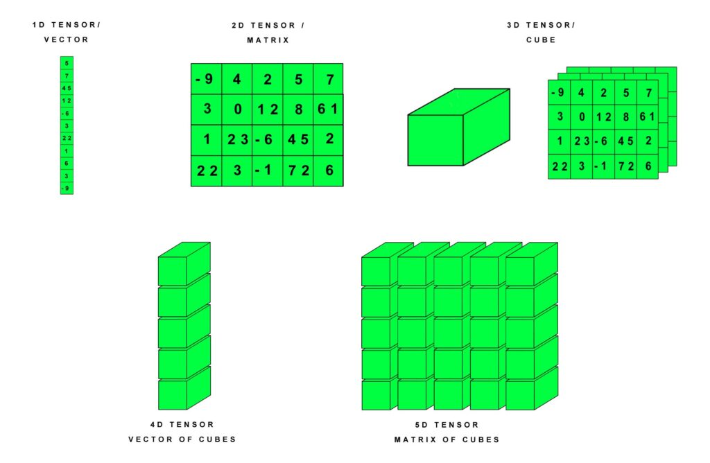
Tensors are used to store a variety of data such as the data neural networks operate on or the parameters of the networks. Tensors can be used in a very similar manner as Python numpy arrays. At the same time, Tensors surpass the capabilities of numpy arrays since they can run either on the CPU or CPU and keep track of gradients.
Tensor Creation
Tensors can be created in a variety of ways.
The content and datatype of a tensor can be directly specified when creating it.
import torch

# create a one dimensional tensor with 3 elements of datatype float64
x = torch.tensor([1.3, 2.5, 1.0], dtype=torch.float64)

# create a two dimensional tensor with 2x2 elements of datatype float32
x = torch.tensor([[1.1, 1.2],[2.1, 2.2]], dtype=torch.float32)
Torch tensors can also be created from other torch tensors. For this, the clone function is provided. This function creates a new tensor with its own memory. If only a regular assignment operator is used, then the new tensor uses the same memory as the original tensor.
import torch

# copy a tensor from another tensor
x = torch.tensor([1.3, 2.5, 1.0], dtype=torch.float64)
y = torch.clone(x)
Alternatively, torch tensors can be created from numpy arrays by using the “from_numpy” function.
import torch
import numpy as np

# copy a tensor from a numpy array
x = np.array([1.3, 2.5, 1.0], dtype=np.float64)
y = torch.from_numpy(x)
Tensors whose elements all have a value of zero or one can be created directly from the corresponding “zeros” and “ones” functions.
import torch

# create a one dimensional tensor with 3 zero values of datatype int32
x = torch.zeros([3], dtype=torch.int32)

# create a two dimensional tensor with 2x2 one values of datatype float32
x = torch.ones([2, 2], dtype=torch.float32)
Tensors can also be created with random values by using the “rand” function. The random values are from a uniform distribution in the interval from 0.0 to 1.0 (excluding 1.0).
import torch

# create a two dimensional tensor with 5x3 random values of datatype float32
x = torch.rand([5, 3], dtype=torch.float32)
When creating a tensor, this tensor initially resides in the memory of the CPU. To conduct tensor operations on the GPU, the tensor has to be moved to the GPU. The member function of the tensor class for moving a tensor from CPU memory to GPU memory (or vice versa) is “to”.
import torch

x = torch.rand([5, 3], dtype=torch.float32)

# move tensor from cpu memory to gpu memory
x = x.to("cuda")

# move tensor from gpu memory to cpu memory
x = x.to("cpu")

# an alternative method for copying a tensor from gpu to cpu memory is to call the member function "cpu" on the tensor
x = x.cpu()

# when creating a new tensor, the move into gpu memory can be done right away.
x = torch.rand([5, 3], dtype=torch.float32).to("cuda")
When transferring a tensor from GPU memory to CPU memory, attention has to be paid on whether the tensor forms part of a computational graph (more about this later on). If that is the case, then the tensor has to be first detached from the computational graph before it can be moved to CPU memory. For this, the member function “detach” can be called on the tensor.
import torch

# assuming that the tensor x exists and has for instance been obtained as output from a model

x = x.detach().cpu()
Tensor Attributes
Tensors possess a variety of attributes that can be accessed for inspection using the corresponding member variables. The tensor attributes that are commonly inspected are dtype, device, and shape.
import torch

x = torch.rand([5, 3], dtype=torch.float32)

# the data type of the values in a tensor is stored in the member variable "dtype"

print(x.dtype)

# the device memory in which the tensor is stored is stored in the member variable "device"

print(x.device)

# one of the most frequently referred to attributes of a tensor is its shape. The shape of a tensor refers to the number of elements along each dimension. The shape can be obtained in the member variable "shape".

print(x.shape)
Casting Tensors
Tensors containing elements of a data type can be casted into tensors containing elements of another data type. For this, the member function “type” can be used.
import torch

x = torch.tensor([5.3, 1.2], dtype=torch.float32)

# cast tensor into a new tensor with a different data type for its elements
y = x.type(torch.float64)
Accessing Tensor Elements
The elements stored in a tensor can be accessed using standard square bracket notation and numerical indices. The calls for accessing the elements are identical to those used for numpy arrays. Accordingly, these calls provide the same level of flexibility for accessing ranges of elements or indexing backwards from the end of a tensor.
import torch

# create a 3x4 tensor with values that make it simple to verify that the correct elements are accessed
x = torch.tensor([[0.0, 0.1, 0.2, 0.3],[1.0, 1.1, 1.2, 1.3],[2.0, 2.1, 2.2, 2.3]], dtype=torch.float32)

# access a scalar element by specifying all indices with indices being counted upwards from zero
x[1, 3]

# access the same scalar element by specifying all indices with indices being counted downwards from the length along each tensor dimension
x[-2, -1]

# access an entire row of values
x[1]

# access an entire column of values
x[:,3]

# access a sub-region of the tensor
x[1:,1:3]
Tensor Mathematical Operations
Basic mathematical operations such as addition, subtraction, multiplication and division are available for tensors. These operations can be conducted between tensors and scalars as well as tensors and tensors.
import torch

x = torch.tensor([1.2, 3.4, 6.1], dtype=torch.float32)
y = torch.tensor([5.1, 0.3, 2.8], dtype=torch.float32)

# mathematical operations between tensor and scalar.
x + 3
x - 10
x * 0.3
x / 2.1

# mathematical operations between tensor and tensor.
x + y
x - y
x * y
x / y
Vector and matrix operations can also available for tensors.
import torch

v1 = torch.tensor([1., 0., 0.], dtype=torch.float64)
v2 = torch.tensor([0., 1., 0.], dtype=torch.float64)
m1 = torch.tensor([[0.0, 0.1],[1.0, 1.1]], dtype=torch.float64)
m2 = torch.tensor([[3.0, 0.0],[0.0, 3.0]], dtype=torch.float64)

torch.cross(v2, v1) # vector cross product
torch.dot(v2, v1) # vector dot product
torch.matmul(m1, m2) # matrix multiplication
torch.svd(m1) # singular value decomposition
Other common mathematical operations include clamping, bitwise operations, comparisons, and reductions.
import torch
import math

x = torch.rand([2, 4], dtype=torch.float64)

# absolute values, rounding, clamping
torch.abs(x) # absolute
torch.ceil(x) # round up
torch.floor(x) # round down
torch.clamp(x, -0.5, 0.5) # clamp

# trigonometric functions
angles = torch.tensor([0, math.pi / 4, math.pi / 2, 3 * math.pi / 4])
torch.sin(angles) # sine
torch.asin(torch.sin(angles)) # inverse sine

# bitwise operations
b = torch.tensor([1, 5, 11], dtype=torch.int32)
c = torch.tensor([2, 7, 10], dtype=torch.int32)
torch.bitwise_xor(b, c) # bitwise xor

# comparisons
torch.eq(b, c) # equality

# reductions
torch.max(x) # maximum value
torch.mean(x) # mean value
torch.std(x) # standard deviation
torch.prod(x) # product
Datasets
Data used for training or inference is organised in datasets. PyTorch offers two classes for this. The Dataset class stores the data and the DataLoader class allows to iterate over the data. These classes offer functions for randomising data, for associating input data and labels, for splitting data into batches, and for pre-processing data. The basic Dataset class needs to be sub-classed to handle any actual data. Pytorch provides convenience classes for dealing with standard datasets and standard types of data (such as images and audio). The following section describes how to work with custom data that involves features and labels. The code example can be easily modified for data that doesn’t have labels.
When writing you own custom Dataset class, there are three functions that need to be implemented. The constructor “__init__” which takes as arguments at least the features and labels that will be stored by the dataset. The function “__len__” which returns the size of the dataset which corresponds to the number of data instances stored in it. The function “__getitem__” which returns a data instance.
import torch
from torch.utils.data import Dataset, DataLoader

# create to random tensors representing dummy data for the dataset
data_count = 100 # number of data instances
data_dim = 8 # number of features per instance
label_count = 4 # number of class labels

dummy_features = torch.rand([data_count, data_dim], dtype=torch.float32)
dummy_labels = torch.randint(0, label_count, [data_count], dtype=torch.int32)

# Create class for a simple customised Dataset by subclassing Dataset
class CustomDataset(Dataset):
    def __init__(self, features, labels):
        self.features = features
        self.labels = labels
    def __len__(self):
        return len(self.features)
    def __getitem__(self, idx):
        feature = self.features[idx]
        label = self.labels[idx]
        return feature, label

# Create an instance of the customised dataset
customDataset = CustomDataset(dummy_features, dummy_labels)

#print length of dataset
print(len(customDataset))

#iterate over all data instances
for instance in iter(customDataset):
    print(instance)
To split a full dataset into two datasets, one for training and one for testing, the torch.utils.data.random_split can be used.
# continuation from previous code block

# split full dataset into train and test dataset

train_test_ratio = 0.8 # 80% of data goes into training set, 20% into test set
train_size = int(len(customDataset) * train_test_ratio)
test_size = len(customDataset) - train_size

train_dataset, test_dataset = torch.utils.data.random_split(customDataset , [train_size, test_size])

print("train dataset size: ", len(train_dataset))
print("test dataset size: ", len(test_dataset))
An instance of the DataLoader class can be created by passing an instance of the Dataset class to the DataLoader constructor. This is the only mandatory argument. Other typically used arguments include “batch_size” and “shuffle”. “Batch_size” specifies the number of data instances in a batch. “Shuffle” specifies if the data instances should be picked randomly from a Dataset. Once a Dataloader has been instantiated, it can be iterated over with each iteration returning a batch of training data.
# continuation from previous code block

# instantiate DataLoaders

batch_size = 16

train_dataloader = DataLoader(train_dataset, batch_size=batch_size, shuffle=True)
test_dataloader = DataLoader(test_dataset, batch_size=batch_size, shuffle=False)

batch = next(iter(train_dataloader))

batch_features = batch[0]
batch_labels = batch[1]

print("batch features shape ", batch_features.shape)
print("batch labels shape", batch_labels.shape)

# iterate over DataLoader for test dataset

for (idx, batch) in enumerate(test_dataloader):
    print("batch ", idx, " features: ", batch[0])
    print("batch ", idx, " labels: ", batch[1])
Network Layers
PyTorch provides a large number of different layer types from which neural networks can be constructed. These layers are accessible via the torch.nn module. This module contains among others conventional neural network layers (torch.nn.Linear), convolution layers (e.g. torch.nn.Conv2d), and recurrent layers (e.g. torch.nn.LSTM). Activation functions are added to a network as separate layers (e.g. torch.nn.ReLU).
A single conventional artificial neural network layer can be created as follows:
import torch
import torch.nn as nn

# create a single classical network layer
input_feature_count = 8
output_feature_count = 1

dummy_layer = nn.Linear(input_feature_count, output_feature_count)

# pass dummy data through layer

batch_size = 16
dummy_input = torch.rand([batch_size, input_feature_count], dtype=torch.float32)
dummy_output = dummy_layer(dummy_input)

print("dummy_input shape ", dummy_input.shape)
print("dummy_output shape ", dummy_output.shape)
A tensor that is passed into a classical artificial neural network layer needs to possess the following shape: batch size x feature count. The feature count needs to match the number of input features specified when creating the layer. The tensor that is output by the layer also has the shape: batch size x feature count. but this time the feature count matches the number of output features that has been specified when creating the layer.
A single 2d convolution layer can be created as follows:
import torch
import torch.nn as nn

# create a single convolutional network layer
input_channel_count = 3 # number of channels in the input feature map
output_channel_count = 8 # number of channels in the output feature map
kernel_size = 5 # 5 x 5 kernel
stride = 2
padding = 0

dummy_layer = nn.Conv2d(input_channel_count, output_channel_count, kernel_size, stride, padding)

# pass dummy data through layer
batch_size = 16
input_size = [64, 64]
dummy_input = torch.rand([batch_size, input_channel_count, input_size[0], input_size[1]], dtype=torch.float32)
dummy_output = dummy_layer(dummy_input)

print("dummy_input shape ", dummy_input.shape)
print("dummy_output shape ", dummy_output.shape)
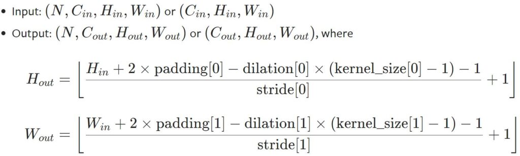
For convolution network layers, the shape of the input tensor is batch size x channel count x feature map height x feature map width. The channel count needs to match the number of input channels specified when creating the layer. The shape of the output tensor is also batch size x channel count x feature map height x feature map width. Here, the channel count corresponds to the number of output channels specified when creating the layer. Calculating the height and width of the output tensor is a bit more involved since it depends not only on the height and width of the input tensor but also on the size of the kernel, the stride, and the padding (and also dilation when used). The equations to calculate the output height and width are as follows:
A single or multiple recurrent layers (LSTM) can be created as follows:
import torch
import torch.nn as nn

# create a LSTM network layer
input_feature_count = 8
hidden_feature_count = 512 # number of features in the hidden state h
layer_count = 2 # number of recurrent layers
batch_first = True

dummy_layer = nn.LSTM(input_feature_count, hidden_feature_count, layer_count, batch_first=batch_first)

# pass dummy data through layer
batch_size = 16
sequence_length = 64
dummy_input = torch.rand([batch_size, sequence_length, input_feature_count], dtype=torch.float32)
dummy_output, (hidden_state, cell_state) = dummy_layer(dummy_input)

print("dummy_input shape ", dummy_input.shape)
print("dummy_output shape ", dummy_output.shape)
print("hidden_state shape ", hidden_state.shape)
print("cell_state shape ", cell_state.shape)
The construction and use of LSTM layers differs significantly from conventional or convolution network layers. First, LSTM layers are typically not constructed one single layer after the other. Instead, the layer constructor takes as argument the number of layers. If this number is larger than one, the constructor automatically creates a stack of LSTM layers. LSTM layers return not only one but three output tensors. The first tensor represents the regular data output. The second tensor contains the hidden states of the layers. The last tensor contains the cell states of the layers. When the batch_first constructor argument is set to False (which is the default value), then the input and output data possess the following shape: sequence length x batch size x feature dimension. If the batch_first argument is set to True, then shape of the input and output data is: batch size x sequence length x feature dimension. The batch_first flag doesn’t affect the shape of the hidden states. These are always: layer count x batch size x hidden feature count. As a side note, another flag that can be specified when creating a stack of LSTM layers is “bidirectional”. The default value is False. If the flag is set to true, the LSTM operates in bidirectional mode which means that the sequence of data runs in both directions, backwards (future to past) and forward (past to future). If this is the case, then the shape of the hidden layer changes to: layer count * 2 x batch size x hidden feature count.
Combining Multiple Network Layers
PyTorch offers different options to combine multiple layers when processing input data. One option is to explicitly pass the output data of one layer as input into the next layer. While this option requires the largest amount of code writing, it also offers the greatest flexibility including for instance conditional passes of data through layers.
# the code assumes that the layers and the tensor containing input data already exist.
# The variables for the layers are named layer0 to layerN and the variable for the input tensor is x.
# Then an explicit forward pass of the input data can be specified as follows:

x = layer0(x) # pass x into 1. layer and assign output tensor to x
x = layer1(x) # pass x into 2. layer and assign output tensor to x
x = layer2(x) # pass x into 3. layer and assign output tensor to x
....
y = layerN(x) # pass x into last layer and assign output tensor to y
Another option is to use the class torch.nn.Sequential. This class serves as sequential container for layers. Layers that are added to an instance of this class are cascaded one after the other. When data is input input into a sequential container, then this data is internally forwarded as input into the first layer, then the output of the first layer is passed as input into the second layer, and so on. The output of the last layer is returned as output of the sequential container.
# the code assumes that the tensor containing input data already exist.

# add all layers to a sequential container

layers = nn.Sequential(
          nn.Conv2d(1,20,5),
          nn.ReLU(),
          nn.Conv2d(20,64,5),
          nn.ReLU()
        )

# directly pass input data into the sequential container

y = layers(x)
A variation of using the class torch.nn.Sequential is to combine it with an instance of an OrderedDict. An OrderedDict is, as the name implies, an ordered dictionary. To such a dictionary, the layers are added as values. The keys could then be used to name the layers. This approach offers two benefits. First, naming the layers makes it easier to identify layers for instance during debugging. Second, the layers can be added using procedures instead of hard-coding them. Such procedures offer the flexibility to compute the number and settings of layers automatically.
# the code assumes that the tensor containing input data already exist.

from collections import OrderedDict

# add all layers to a python list

layer_list = []
layer_list.append(("conv1", nn.Conv2d(1,20,5)))
layer_list.append(("relu1", nn.ReLU()))
layer_list.append(("conv1", nn.Conv2d(20,64,5)))
layer_list.append(("relu1", nn.ReLU()))

# create sequential container from an OrderedDict

layers = nn.Sequential(OrderedDict(layer_list))

# directly pass input data into the sequential container

y = layers(x)
Models
In Pytorch, machine-learning models are created by subclassing the nn.Module class. Doing so involves overwriting the constructor and a forward function of the base class. Typically, the constructor is used to create all layers and the forward function is used to process data with a forward pass. Other than that, the model class inherits from the nn.Module base class functions to switch between training and evaluation mode, and to load previously stored weights.
import torch
import torch.nn as nn
from collections import OrderedDict

# declare model class by subclassing nn.Module
class Model(nn.Module):
    def __init__(self):
        super().__init__()

        layer_list = []
        layer_list.append(("conv1", nn.Conv2d(1,20,5)))
        layer_list.append(("relu1", nn.ReLU()))
        layer_list.append(("conv2", nn.Conv2d(20,64,5)))
        layer_list.append(("relu2", nn.ReLU()))

        self.layers = nn.Sequential(OrderedDict(layer_list))

    def forward(self, x):
        return self.layers(x)

# instantiate model
model = Model()

# print textual summary of model
print(model)

# set model into evaluation mode
model.eval()

# create a test input tensor for the model
batch_size = 16
input_channel_count = 1
input_size = [64, 64]
dummy_input = torch.rand([batch_size, input_channel_count, input_size[0], input_size[1]], dtype=torch.float32)
print("dummy_input shape ", dummy_input.shape)

# conduct a forward pass with the dummy input
dummy_output = model(dummy_input)

# verify shape of output tensor
print("dummy_output shape ", dummy_output.shape)

# set model back into training mode
model.train()

# save model weights
torch.save(model.state_dict(), "model_weights")

# load model weights
model.load_state_dict(torch.load("model_weights"))
A brief note on the evaluation and training modes of models. Changing this mode only has an effect for models that contain certain types of layers such as Dropout layers or BatchNormalisation layers.
Apart from saving and loading model weights, a model can also be saved. Models can be saved in three different formats: in a directly serialised format using Python’s pickle module, in the ONNX (Open Neural Network eXchange) format, or as TorchScript code.
Using pickle is easy but comes with the drawback that the saved model is bound to specific classes and directory structures used when saving the model. Models that are saved in the ONNX format can be used by any of the runtimes that support this format. Models that are saved as Torchscript Saving a model in ONNX format or as TorchScript requires an example of an input tensor that can be processed by the model.
# continuation from previous code block

# save model using pickle
model.eval()
torch.save(model, "model.pth")
model.train()


#load model using pickle
model = torch.load("model.pth")
model.eval()

# save model in ONNX format
model.eval()
torch.onnx.export(model, dummy_input, "model.onnx")
model.train()

# save model as TorchScript
model.eval()
script_module = torch.jit.trace(model, dummy_input)
script_module.save("model.pt")
model.train()
Training an Model
Training a model involves the following steps.
- define a loss function
- instantiate an optimisation algorithm
- iterate through a dataset by conducting the following steps for each batch of data
- forward data through the model
- compute the prediction error using the loss function
- clear gradients for the model weights
- conduct a back propagation step to calculate new gradients
- update the model weights
The torch.optim module provides various optimisation algorithms such as Adam or RMSprop. A list of all available optimisation algorithms is available here.
The torch.nn module provides various predefined loss functions such as Mean Square Error or CrossEntropyLoss. A list of all available loss functions is available here.
# this code assumes that a model and a dataset / dataloader have already been created.

learning_rate = 1e-4
epochs = 10

# instantiate loss function
loss_function = nn.CrossEntropyLoss()

# instantiate optimiser
optimiser = torch.optim.Adam(model.parameters(), lr=learning_rate)

# iterate over all epochs
for epoch in range(epochs):

    # set model into training mode
    model.train()

    train_loss_per_epoch = []

    # iterate over all batches in the train data set
    for batch in train_dataloader:
        batch_features = batch[0].to(device)
        batch_labels = batch[1].to(device)

        # forward pass
        pred_labels = model(batch_features)

        # calculate prediction error
        loss = loss_function(pred_labels, batch_labels)

        # clear gradients
        optimiser.zero_grad()

        # back propagation
        loss.backward()

        # update model weights
        optimiser.step()

        train_loss_per_epoch.append(loss.detach().cpu().numpy())

    train_loss_per_epoch = np.mean(np.array(train_loss_per_epoch))

    print ("epoch {} : train loss: {:01.4f}".format(epoch, train_loss_per_epoch)
It is usually recommended to test a model that is being trained on data from a test dataset. These tests should be done in parallel to the training. In order to ensure that the data from the test dataset doesn’t affect the model weights, it is important to deactivate the calculation of gradients that would normally be automatically conducted by PyTorch. The gradient calculation can be temporarily deactivated by calling the “no_grad” function. Any operations that are executed while the “no_grad” function is active will not cause the gradients to change. Iterating over an entire test dataset can then be implemented for example as follows:
# continuation from previous code block

# iterate over all epochs
for epoch in range(epochs):

    # code for iterating over all batches of the training dataset and updating model weights goes here

    # set model into evaluation mode
    model.eval()

    test_loss_per_epoch = []

    # iterate over all batches in the test data set
    for batch in test_dataloader:
        batch_features = batch[0].to(device)
        batch_labels = batch[1].to(device)

        # deactivate gradient calculation
        with torch.no_grad():
            # forward pass
            pred_labels = model(batch_features)

            # calculate prediction error
            loss = loss_function(pred_labels, batch_labels)

        test_loss_per_epoch.append(loss.detach().cpu().numpy())

    test_loss_per_epoch = np.mean(np.array(test_loss_per_epoch))

    print ("epoch {} : test loss: {:01.4f}".format(epoch, test_loss_per_epoch)


    # set model into training mode
    model.train()
Computational Graphs
A brief note is in place concerning the concept and principle of computational graphs. When processing tensors with a model or any other function, the processing operations take place within a computational graph. A computational graph is a tree structure whose nodes are tensor operations. These operations are connected to each other through directed links. A computation is conducted by passing tensors into the root nodes and then processing them consecutively by following the links. In the case of a forward pass, the links are followed in the direction from input layers to loss function. In case of backpropagation, the links are followed into the opposite direction.
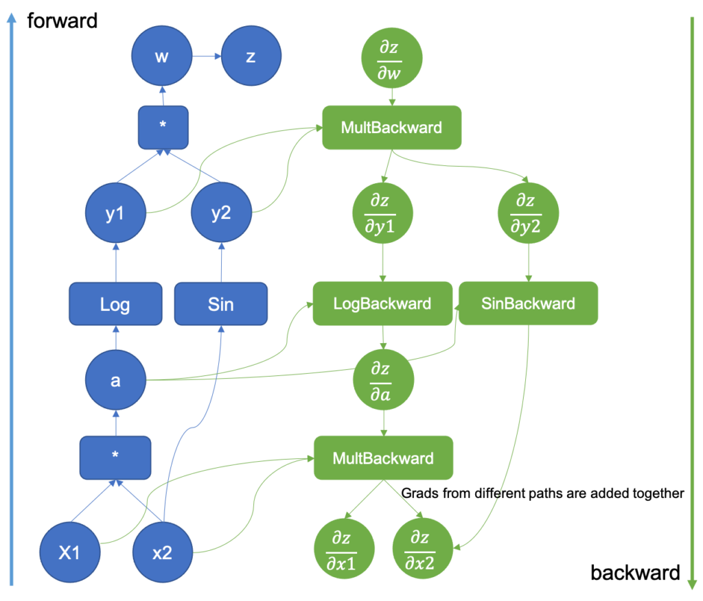
To retrieve tensors that have been created by a computational graph and access their internal values, these tensors have to be detached from the graph. The member function “detach” can be used for this. In case the detached tensor resides in GPU memory, then its content has to be copied into CPU memory before accessing it.