Among the plethora of different machine learning approaches, Deep Learning is currently the one that generates the most excitement and concern. Many of the recent advances in data mining that drive the business of big tech companies are based on applications in Deep Learning. At the same time, Deep Learning has also tremendous artistic potential since it can directly operate on and generate content for digital media.
Deep Learning is a summary term for any approach that employs neural networks that consist of a large number of layers. Many aspects of Deep Learning are therefore inherited from “traditional” artificial neural networks.
Shallow and Deep Neural Networks
Shallow neural networks are networks that possess only a few hidden layers. Deep neural network possess a potentially very large number of hidden layers. The reason why a large number of hidden layers increases the capabilities of a neural network is based on the principle that data can be represented at different levels of abstraction. Lower levels of abstraction are used closer to the input layer, and higher levels of abstraction are used closer to the output layer. Accordingly, deep neural networks can extract features from data at increasingly higher levels of abstraction. Training such a large number of layers has become possible thanks to improvements in learning algorithms and back propagation.

But Deep Learning is more than a simple improvement and upscaling of existing algorithms. Deep Learning has also introduced more diverse network types. This includes network types that are particularly suitable for dealing with temporal data or spatial data. Thanks to these additional network types, Deep Learning can be used in many end-to-end learning scenarios.
End-to-End Learning

Traditional machine learning made it possible to replace some components of a data processing pipeline that were previously programmed by hand with algorithms that are trained on data. Since traditional machine learning models cannot handle high dimensional unstructured data such as raw video images or raw audio, many hand programmed algorithms are still required to pre-process raw data and extract low dimensional features from it. These features can then be passed into a machine learning model. With Deep Learning, machine learning models can be created that are sufficiently powerful to directly deal with raw data. Accordingly, the feature extraction step no longer needs to happen before data is passed into the model. Rather, this step happens within the model and is learned by model alongside all the other data processing aspects during training. Training such a model on raw data is called End-to-End learning.
Recurrent Neural Networks
Conventional artificial neural networks have no notion of time or sequence. These networks don’t take into account the sequence in which data instances are presented to them. Accordingly, these networks cannot learn sequential dependencies and correlations. But such dependencies play an important role in many domains such as language or music. In spoken or written language, it is obvious that the form and choice of a word depends on other words that have appeared earlier in a sentence. Conventional artificial neural networks are not able to capture this.
In order to introduce the notion of time, nodes in a neural network need to be equipped with some sort of memory. The first attempt to do so was to equip conventional artificial neurons with recurrent connections. Such connections pass the output of a neuron back to its input. Accordingly, such neurons “remember” their previous activities since these activities are passed into them alongside with new input data.
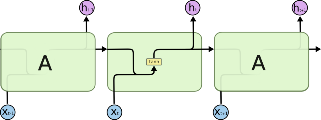
Originally, for neurons that possess a recurrent connection back into themselves, the connection was depicted as a loop. This depiction has been replaced with a form in which the recurrent connection is unrolled in time. In such a depiction, the recurrent connection is shown as a directed arrow that points from the neuron at a previous time step to the same neuron at the next time step.

This type of visualisation highlights one of the main problems of recurrent neural networks, which are long term dependencies between a current output (and its associated error) and an input that possibly lies far back in time. To learn long term dependencies is very difficult for such a network, among others because of they way that gradients are calculated during Back Propagation. The longer the sequence of operations between input and output, the more likely it is that the gradient becomes very small or very large. This is called the vanishing or exploding gradient problem.
Long Short Term Memory Networks
To deal with the problem that conventional recurrent neural networks fail to learn long-term dependencies, a new and more sophisticated type of unit (the term neuron has been abandoned since the design is no longer inspired by biological neurons) has been invented by Hochreiter & Schmidhuber in 1997. Contrary to conventional artificial neurons, these units possess internal states and process these states and new input in a more sophisticated manner.


In a conventional neuron in a recurrent neural network, both the previous cell activity and the current input are combined and passed through a hyperbolic tangent activation function. In a unit in a LSTM network, the internal processing is more complicated. Such a unit possess two states, one state is called Cell State and the other Hidden State. These two states are passed through the recurrent connections instead of a neuron’s activity. Furthermore, the unit employs several gates to determine how large the contribution is of the previous cell states and current input to the new cell states and current output. A forget gate determines based on the previous Hidden State and current input how much of the previous Cell State should be kept. An input gate determines based on the previous Hidden State and current input how much of the current input should be added to the Cell State. An output gate determines based on the previous Hidden State and current input how much Cell State should be passed as output and as new Hidden State. By endowing LSTM units with these states and gating mechanisms, the vanishing and exploding gradient problem has been partially amended.
Convolutional Neural Networks
Convolutional neural networks have been originally invented in the context of computer vision. These networks are particularly suitable for image processing applications. Convolutional neural networks don’t consist of neurons and weighted connections. Instead, they employ convolution kernels.
Convolution
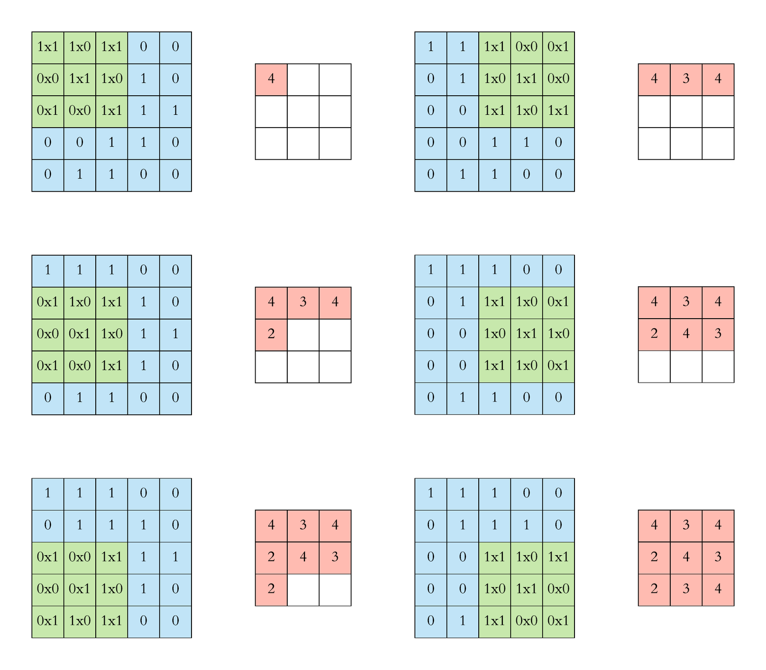
Convolution is a standard method in image (and also audio) processing. In image processing, kernels are used for example for blurring an image or for increasing it’s contrast. When applying convolution to an image, a kernel (a small square matrix) is moved across the image (a large matrix) and at each position, the dot product is calculated between the values of the kernel and the values of the region in the image that is covered by the kernel.

In a convolutional neural network, convolution is employed to extract features from data that is organised in matrices. For each kernel and each matrix, a convolution operation results in the creation of a new matrix. The values in the new matrix represent how much of a feature encoded by a kernel was present in the processed matrix. For this reason, these new matrices are named feature maps.
Convolution Parameters
There exist several parameters that affect how a convolution operation is executed. The most important parameters are Padding and Stride.
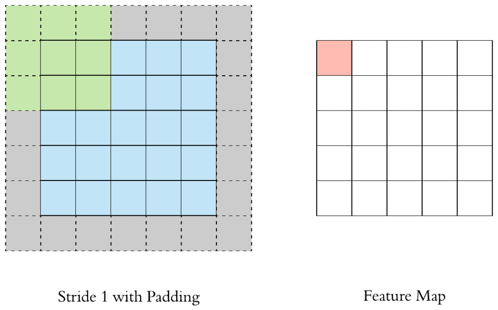
Padding is used to extend the size of a feature map before applying convolution. Such an extension can be achieved by adding columns and rows to the edges of a feature map that either contain zeros or the values at the original edges. By padding a feature map, it can be avoided that the resolution of the new feature map decreases because a kernel doesn’t cover the edges.
Stride refers to the offset that is applied when a kernel traverses a feature map. With a Stride bigger than 1, a kernel skips rows and columns during traversal.


Pooling
Other operations that are frequently used in convolutional neural networks are so called pooling operations. The purpose of pooling is to quickly reduce the size of a feature map while preserving its most important features. Pooling operations are similar to kernels in that they are applied to regions of a feature map by sliding across the map, and in that they output a scalar value for each region of the feature map they are applied to. Pooling operations are different from kernels in that they have no trainable parameters. The following pooling operations are common: max pooling, sum pooling, mean pooling. Max pooling outputs only the highest value in a region and discards all other values. Sum pooling outputs the sum all values in a region. Mean pooling outputs the mean of all values in a region.

Layers and Feature Maps
A Convolutional neural network is organised into layers. Each layer contains a set of feature maps and kernels. From input to output, the number of feature maps typically increases and their resolution decreases. In a Convolutional neural network that is used for classification such as the one depicted below, there is a transition from convolutional layers to conventional layers of an artificial neural network. Since conventional artificial neural network don’t work on data in the form of matrices, the matrices need to be “flattened” into one-dimensional vectors.

Benefits
Convolutional neural networks possess two main benefits over conventional neural networks. First, they take into account the spatial characteristics of the data they operate on. This allows them to exploit for example the fact that regions in an image that are close together are typically more similar to each other than those that are further apart. Second, kernels represent the trainable parameters. Since kernels are shared across all the regions of a feature map, the number of trainable parameters is much lower than if each value in a feature map would be associated with a conventional neuron which possesses connections to each neuron in the next feature map.