Image Generation with an Adversarial Autoencoder

Summary

The following tutorial introduces the use of an adversarial autoencoder model for generating synthetic images. This model can be trained on a collection of images. The model uses a combination of a conventional neural network (ANN) and a convolutional neural network (CNN) to create images. Apart from explaining how to create and train the corresponding models, this article also provides some examples how the latent space of image encodings can be navigated to discover potentially interesting synthetic images.

This tutorial forms part of a series of tutorials on using PyTorch to create and train generative deep learning models. The code for these tutorials is available here.

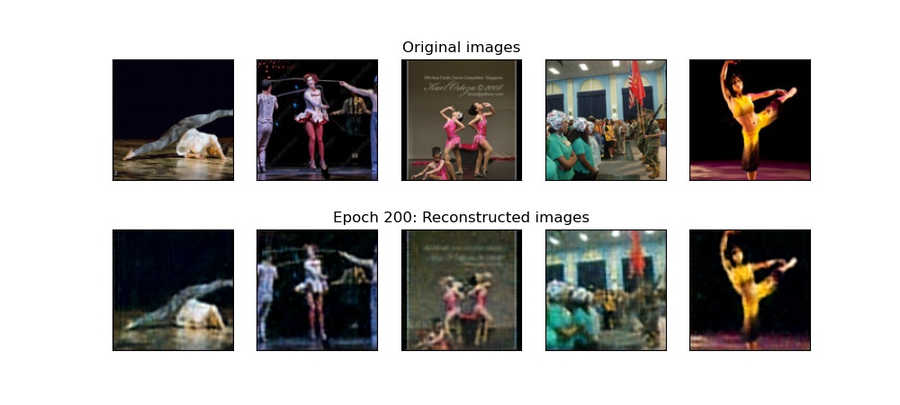
After 200 epochs of training, the images reconstructed by the autoencoder look like this.

Create Models

The code parts for importing images from a local directory and creating Datasets and Dataloaders for training and testing are identical to those in a previous article on Image Generation with a GAN. These code parts are skipped here.

An adversarial autoencoder (AAE) consists of three models. A model named Encoder that compresses input data into a latent vector, a model named Decoder that recreates the input data from the latent vector, and a model named Discriminator, that distinguishes between random variables from a true normal distribution and the latent vectors. A brief introduction into autoencoders is available here.

In this example, the models operate on images. The Encoder and Decoder models employ as networks a combination of convolutional neural networks (CNN) and conventional artificial neural networks (ANN). The Discriminator model employs an ANN only.

Create Discriminator Model

The Discriminator model classifies latent vectors as random variables that either have been sampled from a true normal distribution or that have ben created by the Encoder. For converting input latent vectors into output classes, the Discriminator passes the latent vectors through several ANN layers. These layers successively reduce the dimension of the latent vectors down to 1. Each ANN layer with the exception of the last one is followed by a Exponential Linear Unit (ELU) activation function. The last ANN layer is followed by a Softmax activation function to obtain normalised class probabilities.

The class definition of the Discriminator model is as follows:

class DiscriminatorPrior(nn.Module):
    def __init__(self, latent_dim, dense_layer_sizes):
        super().__init__()
        
        self.latent_dim = latent_dim
        self.dense_layer_sizes = dense_layer_sizes
        
        # create dense layers
        dense_layers = []
        
        dense_layers.append(("disc_prior_dense_0", nn.Linear(latent_dim, dense_layer_sizes[0])))
        dense_layers.append(("disc_prior_elu_0", nn.ELU()))
        
        dense_layer_count = len(dense_layer_sizes)

        for layer_index in range(1, dense_layer_count):
            dense_layers.append( ( "disc_prior_dense_{}".format( layer_index ), nn.Linear( dense_layer_sizes[layer_index - 1], dense_layer_sizes[layer_index] ) ) )
            dense_layers.append(("disc_prior_elu_{}".format(layer_index), nn.ELU()))
    
        dense_layers.append( ( "disc_prior_dense_{}".format( dense_layer_count ), nn.Linear(dense_layer_sizes[-1], 1) ) )
        dense_layers.append( ( "disc_prior_sigmoid_{}".format( dense_layer_count ), nn.Sigmoid() ) )
        
        self.dense_layers = nn.Sequential(OrderedDict(dense_layers))
        
    def forward(self, x):
        
        #print("x1 s", x.shape)
        
        yhat = self.dense_layers(x)
        
        #print("yhat s", yhat.shape)
        
        return yhat

The constructor of the Discriminator model class takes two arguments: the latent dimension and a sequence of unit counts for the ANN layers (with the unit count of 1 for the last layer missing, since this layer is added anyway). The Discriminator model class can be instantiated as follows:

latent_dim = 64
disc_prior_dense_layer_sizes = [ 128, 128 ]

disc_prior = DiscriminatorPrior(latent_dim, disc_prior_dense_layer_sizes).to(device)

The shapes of the input and output tensors for this model are as follows:

input tensor: batch_size x latent_dim
output tensor: batch_size x 1

Create Encoder Model

For compressing images into a one dimensional latent vector, the Encoder model first passes the input image through several convolution layers, then flattens the output of the last convolution layer into a one dimensional vector. This vector is then passed through several ANN layers with the last one outputting the latent vector.

The CNN part of the model successively decreases the size of the feature maps while increasing their number of channels. Each convolution layer is followed by a leaky ReLU activation function and a batch normalisation.

The ANN part of the model successively reduces the dimension of the one-dimensional feature vector down to the latent dimension. Each ANN layer with the exception of the last one is followed by a leaky ReLU activation function.

The class definition of the encoder model is as follows:

class Encoder(nn.Module):
    
    def __init__(self, latent_dim, image_size, image_channels, conv_channel_counts, conv_kernel_size, dense_layer_sizes):
        super().__init__()
        
        self.latent_dim = latent_dim
        self.image_size = image_size
        self.image_channels = image_channels
        self.conv_channel_counts = conv_channel_counts
        self.conv_kernel_size = conv_kernel_size
        self.dense_layer_sizes = dense_layer_sizes
        
        # create convolutional layers
        conv_layers = []
        
        stride = (self.conv_kernel_size - 1) // 2
        padding = stride
        
        conv_layers.append(("encoder_conv_0", nn.Conv2d(self.image_channels, conv_channel_counts[0], self.conv_kernel_size, stride=stride, padding=padding)))
        conv_layers.append(("encoder_lrelu_0", nn.LeakyReLU(0.2)))
        conv_layers.append(("encoder_bnorm_0", nn.BatchNorm2d(conv_channel_counts[0])))
        
        conv_layer_count = len(conv_channel_counts)
        for layer_index in range(1, conv_layer_count):
            conv_layers.append(("encoder_conv_{}".format(layer_index), nn.Conv2d(conv_channel_counts[layer_index-1], conv_channel_counts[layer_index], self.conv_kernel_size, stride=stride, padding=padding)))
            conv_layers.append(("encoder_lrelu_{}".format(layer_index), nn.LeakyReLU(0.2)))
            conv_layers.append(("encoder_bnorm_{}".format(layer_index), nn.BatchNorm2d(conv_channel_counts[layer_index])))

        self.conv_layers = nn.Sequential(OrderedDict(conv_layers))
        
        self.flatten = nn.Flatten()
        
        # create dense layers
        dense_layers = []
        
        last_conv_layer_size = int(image_size // np.power(2, len(conv_channel_counts)))
        preflattened_size = [conv_channel_counts[-1], last_conv_layer_size, last_conv_layer_size]
        dense_layer_input_size = conv_channel_counts[-1] * last_conv_layer_size * last_conv_layer_size
        
        dense_layers.append(("encoder_dense_0", nn.Linear(dense_layer_input_size, self.dense_layer_sizes[0])))
        dense_layers.append(("encoder_relu_0", nn.ReLU()))
        
        dense_layer_count = len(dense_layer_sizes)
        for layer_index in range(1, dense_layer_count):
            dense_layers.append(("encoder_dense_{}".format(layer_index), nn.Linear(self.dense_layer_sizes[layer_index-1], self.dense_layer_sizes[layer_index])))
            dense_layers.append( ( "encoder_dense_relu_{}".format( layer_index ), nn.ReLU() ) )
    
        dense_layers.append( ( "encoder_dense_{}".format( len( self.dense_layer_sizes ) ), nn.Linear( self.dense_layer_sizes[-1], self.latent_dim ) ) )
        
        self.dense_layers = nn.Sequential(OrderedDict(dense_layers))

    def forward(self, x):
        
        #print("x1 s ", x.shape)
        
        x = self.conv_layers(x)
        
        #print("x2 s ", x.shape)
        
        x = self.flatten(x)
        
        #print("x3 s ", x.shape)

        yhat = self.dense_layers(x)
        
        #print("yhat s ", yhat.shape)

        return yhat

The constructor of the Encoder model class takes the following arguments: the latent dimension, the size of a square image, the number of image channels, a sequence of channel counts for the convolution layers, the size of the convolution kernels, and a sequence of unit counts for the ANN layers (with the unit count equal to the latent dimensions for the last layer missing, since this layer is added anyway). The Encoder model class can be instantiated as follows:

image_size = 128
image_channels = 3
ae_conv_channel_counts = [ 8, 32, 128, 512 ]
ae_conv_kernel_size = 5
ae_dense_layer_sizes = [ 128 ]

encoder = Encoder(latent_dim, image_size, image_channels, ae_conv_channel_counts, ae_conv_kernel_size, ae_dense_layer_sizes).to(device)

The shapes of the input and output tensors for this model are as follows:

input tensor: batch_size x image_channels x image_size x image_size
output tensor: batch_size x latent_dim

Create Decoder Model

The Decoder model mirrors the task and network structure of the Encoder model. For decompressing a one dimensional latent vector, the Decoder model first passes the latent vector though several ANN layers, then un-flattens the output of the last ANN layer into a two-dimensional feature map. This feature map is then passed through several deconvolution layers with the last one outputting a reconstructed image.

The ANN part of the model successively increases the dimension of the latent dimension vector. Each ANN layer is followed by a ReLU activation function.

The CNN part of the model successively increases the size of the feature maps while decreasing their number of channels. Each deconvolution layer is preceded by a batch normalisation and followed by a leaky ReLU activation function.

The class definition of the Decoder model is as follows:

class Decoder(nn.Module):
    
    def __init__(self, latent_dim, image_size, image_channels, conv_channel_counts, conv_kernel_size, dense_layer_sizes):
        super().__init__()
        
        self.latent_dim = latent_dim
        self.image_size = image_size
        self.image_channels = image_channels
        self.conv_channel_counts = conv_channel_counts
        self.conv_kernel_size = conv_kernel_size
        self.dense_layer_sizes = dense_layer_sizes
        
        # create dense layers
        dense_layers = []
                
        dense_layers.append(("decoder_dense_0", nn.Linear(latent_dim, self.dense_layer_sizes[0])))
        dense_layers.append(("decoder_relu_0", nn.ReLU()))
        
        dense_layer_count = len(dense_layer_sizes)
        for layer_index in range(1, dense_layer_count):
            dense_layers.append(("decoder_dense_{}".format(layer_index), nn.Linear(self.dense_layer_sizes[layer_index-1], self.dense_layer_sizes[layer_index])))
            dense_layers.append( ( "decoder_dense_relu_{}".format( layer_index ), nn.ReLU() ) )
            
        last_conv_layer_size = int(image_size // np.power(2, len(conv_channel_counts)))
        preflattened_size = [conv_channel_counts[0], last_conv_layer_size, last_conv_layer_size]
        dense_layer_output_size = conv_channel_counts[0] * last_conv_layer_size * last_conv_layer_size

        dense_layers.append( ( "decoder_dense_{}".format( len( self.dense_layer_sizes ) ), nn.Linear( self.dense_layer_sizes[-1], dense_layer_output_size ) ) )
        dense_layers.append( ( "decoder_dense_relu_{}".format( len( self.dense_layer_sizes ) ), nn.ReLU() ) )
        
        self.dense_layers = nn.Sequential(OrderedDict(dense_layers))
        
        self.unflatten = nn.Unflatten(dim=1, unflattened_size=preflattened_size)
        
        # create convolutional layers
        conv_layers = []
        
        stride = (self.conv_kernel_size - 1) // 2
        padding = stride
        output_padding = 1
        
        conv_layer_count = len(conv_channel_counts)
        for layer_index in range(1, conv_layer_count):
            conv_layers.append(("decoder_bnorm_{}".format(layer_index), nn.BatchNorm2d(conv_channel_counts[layer_index-1])))
            conv_layers.append(("decoder_conv_{}".format(layer_index), nn.ConvTranspose2d(conv_channel_counts[layer_index-1], conv_channel_counts[layer_index], self.conv_kernel_size, stride=stride, padding=padding, output_padding=output_padding)))
            conv_layers.append(("decoder_lrelu_{}".format(layer_index), nn.LeakyReLU(0.2)))
            
        conv_layers.append(("decoder_bnorm_{}".format(conv_layer_count), nn.BatchNorm2d(conv_channel_counts[-1])))
        conv_layers.append(("decoder_conv_{}".format(conv_layer_count), nn.ConvTranspose2d(conv_channel_counts[-1], self.image_channels, self.conv_kernel_size, stride=stride, padding=padding, output_padding=output_padding)))
        
        self.conv_layers = nn.Sequential(OrderedDict(conv_layers))

    def forward(self, x):
        
        #print("x1 s ", x.shape)
        
        x = self.dense_layers(x)
        
        #print("x2 s ", x.shape)
        
        x = self.unflatten(x)
        
        #print("x3 s ", x.shape)

        yhat = self.conv_layers(x)
        
        #print("yhat s ", yhat.shape)

        return yhat

The constructor of the decoder model class takes the following arguments: the latent dimension, the size of a square image, the number of image channels, a sequence of channel counts for the deconvolution layers, the size of the deconvolution kernels, and a sequence of unit counts for the ANN layers (with the unit count equal to the latent dimensions for the first layer missing since this layer is added anyway). The channel counts for the deconvolution layers and the unit counts for the ANN layers are obtained by reversing the corresponding lists that were used for creating the Encoder model. The Decoder model class can be instantiated as follows:

ae_conv_channel_counts_reversed = ae_conv_channel_counts.copy()
ae_conv_channel_counts_reversed.reverse()
    
ae_dense_layer_sizes_reversed = ae_dense_layer_sizes.copy()
ae_dense_layer_sizes_reversed.reverse()

decoder = Decoder(latent_dim, image_size, image_channels, ae_conv_channel_counts_reversed, ae_conv_kernel_size, ae_dense_layer_sizes_reversed).to(device)

The shapes of the input and output tensors for this model are as follows:

input tensor: batch_size x latent_dim
output tensor: batch_size x image_channels x image_size x image_size

Optimisers and Loss Functions

To update the weights of the three models during training, two individual Adam optimisers are used. One optimiser changes the combined weights of the Encoder and Decoder models. The other optimiser changes only the weights of the Discriminator model. In this example, the optimiser for the Discriminator uses a five times higher learning rate that that for the Encoder/Decoder. These optimisers are instantiated as follows:

dp_learning_rate = 5e-4
ae_learning_rate = 1e-4

disc_prior_optimizer = torch.optim.Adam(disc_prior.parameters(), lr=dp_learning_rate)
ae_optimizer = torch.optim.Adam(list(encoder.parameters()) + list(decoder.parameters()), lr=ae_learning_rate)

Two different loss function are used, one for the Discriminator model and one for the combined Encoder and Decoder models.

The loss function for the Discriminator is based on binary cross-entropy to quantify the classification error. This loss function is almost identical with the one used for the critique model in the articles on generative adversarial networks with the only difference that a version of binary cross-entropy is used that is combined with a sigmoid function. This loss function is defined as follows:

bce_loss = nn.BCEWithLogitsLoss()

def disc_prior_loss(disc_real_output, disc_fake_output):
    _real_loss = bce_loss(disc_real_output, torch.ones_like(disc_real_output).to(device))
    _fake_loss = bce_loss(disc_fake_output, torch.zeros_like(disc_fake_output).to(device))

    _total_loss = (_real_loss + _fake_loss) * 0.5
    return _total_loss

The loss function for the Encoder/Decoder employs a mean squared error to quantify the image reconstruction error. This loss function also takes into account the mistakes the Discriminator makes when classifying latent vectors generated by the Encoder. These two loss components are weighted and summed to obtain a single loss. The loss function for the Encoder and Decoder is defined as follows:

ae_rec_loss_scale = 1.0
ae_prior_loss_scale = 0.1

mse_loss = torch.nn.MSELoss()

def ae_loss(y, yhat, disc_pior_fake_output):
    _ae_rec_loss = mse_loss(y, yhat)
    _disc_prior_fake_loss = bce_loss(disc_pior_fake_output, torch.ones_like(disc_pior_fake_output).to(device))
    
    _total_loss = 0.0
    _total_loss += _ae_rec_loss * ae_rec_loss_scale
    _total_loss += _disc_prior_fake_loss * ae_prior_loss_scale
    
    return _total_loss, _ae_rec_loss, _disc_prior_fake_loss

Finally, a simple function is defined for sampling from a normal distribution. This function provides the Discriminator with true random variables. The sampling function is defined as follows:

def sample_normal(shape):
    return torch.tensor(np.random.normal(size=shape), dtype=torch.float32).to(device)

Training and Testing Functions

A total of three different functions are defined for conducting training and testing steps. A training step function for the Discriminator model and a training and testing step function for the combined Encoder and Decoder models. The function for the Discriminator model is named “disc_prior_train_step” and takes as input a tensor representing a batch of images. The functions for the combined Encoder and Decoder models are named “ae_train_step” and “ae_test_step” and take as input also a tensor representing a batch of images. All these functions compute and return loss values. The functions used for training also calculate the gradients of the loss functions and update the trainable parameters of the corresponding models. The functions used for testing suppresse gradient calculation and leave the trainable model parameters unchanged.

def disc_prior_train_step(target_images):
    # have normal distribution and encoder produce real and fake outputs, respectively
    
    with torch.no_grad():
        encoder_output = encoder(target_images)
        
    real_output = sample_normal(encoder_output.shape)
    
    # let discriminator distinguish between real and fake outputs
    disc_real_output =  disc_prior(real_output)
    disc_fake_output =  disc_prior(encoder_output)   
    _disc_loss = disc_prior_loss(disc_real_output, disc_fake_output)
    
    # Backpropagation
    disc_prior_optimizer.zero_grad()
    _disc_loss.backward()
    disc_prior_optimizer.step()
    
    return _disc_loss

def ae_train_step(target_images):
    
    encoder_output = encoder(target_images)
    pred_images = decoder(encoder_output)

    disc_fake_output = disc_prior(encoder_output)
    
    _ae_loss, _ae_rec_loss, _disc_prior_fake_loss = ae_loss(target_images, pred_images, disc_fake_output) 

    ae_optimizer.zero_grad()
    _ae_loss.backward()
    ae_optimizer.step()
    
    return _ae_loss, _ae_rec_loss, _disc_prior_fake_loss

def ae_test_step(target_images):

    with torch.no_grad():
        encoder_output = encoder(target_images)
        pred_images = decoder(encoder_output)
        disc_fake_output = disc_prior(encoder_output)
    
        _ae_loss, _ae_rec_loss, _disc_prior_fake_loss = ae_loss(target_images, pred_images, disc_fake_output) 
    
    return _ae_loss, _ae_rec_loss, _disc_prior_fake_loss

The function named “train” performs the actual training of the two models by calling the train and test step functions repeatedly. This function takes as arguments the train and test Dataloaders and the number of epochs. It then runs through an outer loop and two inner loops. The outer loop iterates over all epochs. The first inner loop iterates over all the batches provided by the train Dataloader, The second inner loop iterates over all the batches provided by the test Dataloader. In each of these inner loops, the loss returned by the loss functions are added to a dictionary. This dictionary contains the history of the training process. The training function is defined as follows:

def train(train_dataloader, test_dataloader, epochs):
    
    loss_history = {}
    loss_history["ae train"] = []
    loss_history["ae test"] = []
    loss_history["ae rec"] = []
    loss_history["ae prior"] = []
    loss_history["disc prior"] = []
    
    for epoch in range(epochs):

        start = time.time()
        
        ae_train_loss_per_epoch = []
        ae_rec_loss_per_epoch = []
        ae_prior_loss_per_epoch = []
        disc_prior_loss_per_epoch = []
        
        for train_batch, _ in train_dataloader:
            train_batch = train_batch.to(device)

            # start with discriminator training
            _disc_prior_train_loss = disc_prior_train_step(train_batch)
            _disc_prior_train_loss = _disc_prior_train_loss.detach().cpu().numpy()
            disc_prior_loss_per_epoch.append(_disc_prior_train_loss)
            
            # now train the autoencoder
            _ae_loss, _ae_rec_loss, _ae_prior_loss = ae_train_step(train_batch)
            
            _ae_loss = _ae_loss.detach().cpu().numpy()
            _ae_rec_loss = _ae_rec_loss.detach().cpu().numpy()
            _ae_prior_loss = _ae_prior_loss.detach().cpu().numpy()
            
            ae_train_loss_per_epoch.append(_ae_loss)
            ae_rec_loss_per_epoch.append(_ae_rec_loss)
            ae_prior_loss_per_epoch.append(_ae_prior_loss)
        
        ae_train_loss_per_epoch = np.mean(np.array(ae_train_loss_per_epoch))
        ae_rec_loss_per_epoch = np.mean(np.array(ae_rec_loss_per_epoch))
        ae_prior_loss_per_epoch = np.mean(np.array(ae_prior_loss_per_epoch))
        disc_prior_loss_per_epoch = np.mean(np.array(disc_prior_loss_per_epoch))
        
        ae_test_loss_per_epoch = []
        
        for test_batch, _ in test_dataloader:
            test_batch = test_batch.to(device)
            
            _ae_loss, _, _ = ae_test_step(train_batch)
            
            _ae_loss = _ae_loss.detach().cpu().numpy()
            ae_test_loss_per_epoch.append(_ae_loss)
        
        ae_test_loss_per_epoch = np.mean(np.array(ae_test_loss_per_epoch))
        
        if epoch % weight_save_interval == 0 and save_weights == True:
            torch.save(disc_prior.state_dict(), "results/weights/disc_prior_weights_epoch_{}".format(epoch))
            torch.save(encoder.state_dict(), "results/weights/encoder_weights_epoch_{}".format(epoch))
            torch.save(decoder.state_dict(), "results/weights/decoder_weights_epoch_{}".format(epoch))
        
        plot_ae_outputs(encoder, decoder, epoch)
        
        loss_history["ae train"].append(ae_train_loss_per_epoch)
        loss_history["ae test"].append(ae_test_loss_per_epoch)
        loss_history["ae rec"].append(ae_rec_loss_per_epoch)
        loss_history["ae prior"].append(ae_prior_loss_per_epoch)
        loss_history["disc prior"].append(disc_prior_loss_per_epoch)
        
        print ('epoch {} : ae train: {:01.4f} ae test: {:01.4f} disc prior {:01.4f} rec {:01.4f} prior {:01.4f} time {:01.2f}'.format(epoch + 1, ae_train_loss_per_epoch, ae_test_loss_per_epoch, disc_prior_loss_per_epoch, ae_rec_loss_per_epoch, ae_prior_loss_per_epoch, time.time()-start))
    
    return loss_history

To visually verify the progress of the training, the training function calls after each epoch a convenience function named “plot_ae_outputs”. This function uses the autoencoder to reconstruct several images from the test dataset. This function then creates an image in which the original images and the reconstructed images are arranged in a top and bottom row, respectively. The function takes as arguments the Encoder model, Decoder model, the current epoch, and the number of images that should be reconstructed. This function is defined as follows.

def plot_ae_outputs(encoder, decoder, epoch, n=5):
    
    encoder.eval()
    decoder.eval()
    
    plt.figure(figsize=(10,4.5))
    for i in range(n):
      ax = plt.subplot(2,n,i+1)
      img = test_dataset[i][0].unsqueeze(0).to(device)

      with torch.no_grad():
         rec_img  = decoder(encoder(img))    
      
      img = img.cpu().squeeze().numpy()
      img = np.clip(img, 0.0, 1.0)
      img = np.moveaxis(img, 0, 2)
      
      rec_img = rec_img.cpu().squeeze().numpy()
      rec_img = np.clip(rec_img, 0.0, 1.0)
      rec_img = np.moveaxis(rec_img, 0, 2)
      
      plt.imshow(img)
      ax.get_xaxis().set_visible(False)
      ax.get_yaxis().set_visible(False)  
      if i == n//2:
        ax.set_title('Original images')
      ax = plt.subplot(2, n, i + 1 + n)
      plt.imshow(rec_img)  
      ax.get_xaxis().set_visible(False)
      ax.get_yaxis().set_visible(False)  
      if i == n//2:
         ax.set_title("Epoch {}: Reconstructed images".format(epoch))
    plt.show()
    plt.savefig("epoch_{0:05d}.jpg".format(epoch))
    plt.close()
    
    decoder.train()
    decoder.train()

The “train” function can be called as follows:

epochs = 800

loss_history = train(train_dataloader, test_dataloader, epochs)

Generate and Visualise Images

Once the autoencoder has been trained, it can be used to experiment with image reconstruction. For example, a visual comparison can be conducted between how well the autoencoder reconstructs images from the test dataset and training dataset. This can be done as follows:

test_img, _ = test_dataset[0]
train_img, _ = train_dataset[0]

plt.imshow(np.moveaxis(test_img.numpy(), 0, 2))
plt.imshow(np.moveaxis(train_img.numpy(), 0, 2))

test_img = torch.unsqueeze(test_img, 0)
train_img = torch.unsqueeze(train_img, 0)

encoder.eval()
decoder.eval()
with torch.no_grad():
    rec_test_img = decoder(encoder(test_img.to(device)))
    rec_train_img = decoder(encoder(train_img .to(device)))
encoder.train()
decoder.train()

rec_test_img = rec_test_img .cpu().detach().numpy().squeeze()
rec_train_img = rec_train_img .cpu().detach().numpy().squeeze()

plt.imshow(np.moveaxis(rec_test_img , 0, 2))
plt.imshow(np.moveaxis(rec_train_img, 0, 2))

A potentially more interesting thing to do with a trained autoencoder is to experiment with the mixing of latent encodings of images and then decode these mixed encodings into a new images.

mix_factor = 0.5

img_1, _ = train_dataset[0]
img_2, _ = train_dataset[4]

plt.imshow(np.moveaxis(img_1.numpy(), 0, 2))
plt.imshow(np.moveaxis(img_2.numpy(), 0, 2))

img_1 = torch.unsqueeze(img_1, 0)
img_2 = torch.unsqueeze(img_2, 0)

encoder.eval()
with torch.no_grad():
    img_encoding_1 = encoder(img_1.to(device))
    img_encoding_2 = encoder(img_2.to(device))
decoder.train()

mixed_encoding = img_encoding_1 * mix_factor + img_encoding_2 * (1.0 - mix_factor)

decoder.eval()
with torch.no_grad():
    mixed_img = decoder(mixed_encoding)
decoder.train()

mixed_img = mixed_img.cpu().detach().numpy().squeeze()

plt.imshow(np.moveaxis(mixed_img, 0, 2))

Using the same approach as before, a sequence of images can be created by gradually interpolating between the encodings of two images.

img_1, _ = train_dataset[0]
img_2, _ = train_dataset[4]

img_1 = torch.unsqueeze(img_1, 0)
img_2 = torch.unsqueeze(img_2, 0)

encoder.eval()
decoder.eval()

with torch.no_grad():
    img_encoding_1 = encoder(img_1.to(device))
    img_encoding_2 = encoder(img_2.to(device))

mix_index = 0

for mix_factor in np.linspace(0.0, 1.0, 100):
    mixed_encoding = img_encoding_1 * mix_factor + img_encoding_2 * (1.0 - mix_factor)
    
    with torch.no_grad():
        mixed_img = decoder(mixed_encoding)
    
    mixed_img = mixed_img.cpu().detach().numpy().squeeze()
    
    mixed_img = np.clip(mixed_img, 0.0, 1.0)

    #mixed_img = np.clip(mixed_img, 0.0, 1.0)
    mixed_img = np.moveaxis(mixed_img, 0, 2)
    
    plt.imshow(mixed_img)
    plt.savefig("mixed_{0:05d}.jpg".format(mix_index))
    
    mix_index += 1
    
encoder.train()
decoder.train()

Recent Posts

Recent Comments

Archives

Categories

Image Generation with an Adversarial Autoencoder

Summary

Create Models

Create Discriminator Model

Create Encoder Model

Create Decoder Model

Optimisers and Loss Functions

Training and Testing Functions

Generate and Visualise Images