This article plays is a preamble to the other articles since it addresses not a specific simulation technique but rather general methods that are required for implementing simulations on a computer. The simulation that are described in the following articles employ mathematical equations to calculate physical forces. In order for these forces to exert any effects on the simulated objects, the objects’ acceleration, velocities and positions need to be derived from the forces.
Newton’s Second Law of Motion
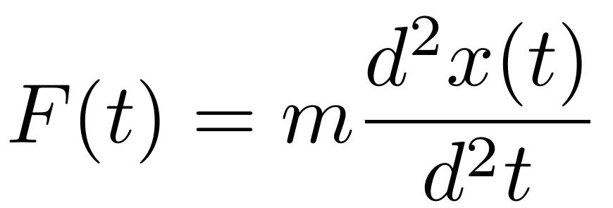
Accelerations can be derived from forces according to Newton’s second law of motion. This law simply states that the force acting on an object is proportional to the object’s acceleration with the proportionality factor being the mass of the object.
Temporal Derivatives
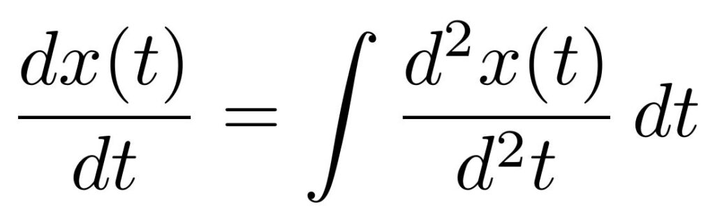
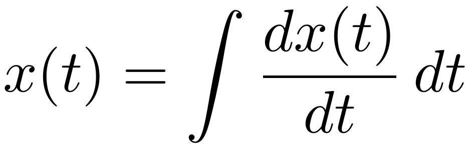
Once the acceleration of an object is known, the object’s velocity and position can be obtained through integration with regards to time. These two equations are very similar. To obtain an object’s velocity, its acceleration is integrated with regards to time, and to obtain an object’s position, it’s velocity is integrated with regards to time.
Numerical Integration
These integral equations treat the physical properties of objects such as position and velocity as symbols and time as continuous parameter. In order to use these equations in a computer simulation, symbols have to be replaced by actual numerical values and time proceeds in discrete steps. This is where numerical integration methods come in. They operate on numerical values and they calculate these values at discrete time intervals.
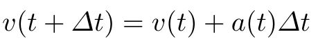
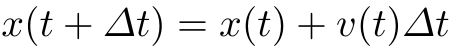
The simplest but also the least stable numerical integration method is the Euler Method. This method employs a piecewise linear approximation by calculating the change of a variable with regards to time at a specific point point in time and then assuming that this change is constant for a certain interval of time.
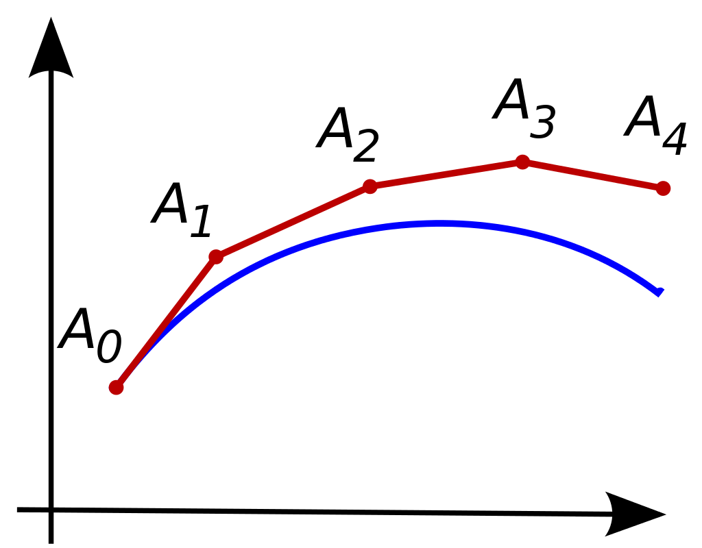
Following this principle, the value of a physical variable such as velocity is obtained from its derivative by taking the value of velocity at some previous point in time and adding to it the value of its derivative at the current point in time multiplied by the interval between the previous and current point in time.
The advantage of the Euler method is that it is very simple to implement and fast to compute. Its disadvantage is its inaccuracy. As can be seen in the figure depicting an approximation, calculations conducted with the Euler method can lead to values that become increasingly more incorrect over time.
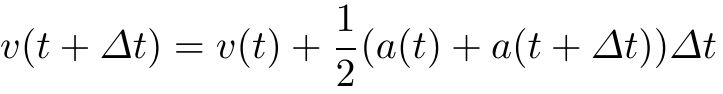
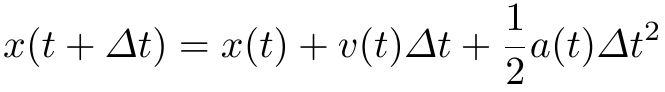
The Leapfrog Method is an alternative integration scheme that is still easy to implement and fast to compute but exhibits much higher numerical stability than the Euler method. The reason for this is twofold: the it employs second order integration instead of only first order as the Euler method, it calculates updated velocities and positions at interleaved times instead of the same times as in the Euler method.
There exist much more sophisticated numerical integration methods than those two that have been described here. An example are the popular Runge–Kutta methods. These methods are used in applications in which numerical stability and accuracy are important. While numerical stability might be of a concern when using simulations for artistic purposes, accuracy is much less so. For these applications, the Leapfrog method is very well suited.