Reinforcement Learning (RL) is a Machine Learning approach that is inspired by how animals or young children learn from their mistakes (or successes). This approach combines trial and error actions with a reward. A typical natural example of this type of learning would be a young child who touches the door of a hot oven and burns his or her fingers. The pain sensation from getting burnt represents a strong negative reward that will likely cause the child to avoid touching hot oven doors from now on.
This type of learning is often applied for agent-based simulations in which an agent needs to develop a strategy for successfully interacting with an environment. The level of success is measured as a reward that an agent receives from the environment after performing an action. This reward can be positive or negative (a punishment) and it can be received instantaneously or in the future. One of the main challenges of RL concerns the correct attribution of rewards to actions when the actions lie far in the past.
Agent, Environment, Action, State, Reward
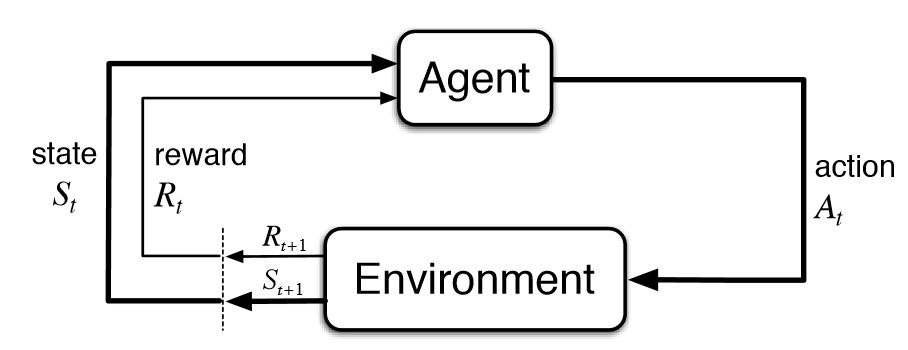
A RL system includes the following elements: Environment, Agent, State, Observation, Action, Reward. The environment represents the world within which the agent acts. The world and the agent have at each point in time a particular state. An agent represents the entity that interacts with the environment and tries to maximise its reward. An agent can observe the environment. Depending on the implementation, such an observation is identical with the state of the environment or it is different. When it is different, then an observation might reveal to the agent only partial information about the environment’s state. Based on this observation, the agent choses an action. An action is an activity conducted by the agent that might cause a change in the state of the environment. Once an action has been executed, the environment responds to it by returning to the agent a reward value and by assuming a new state.
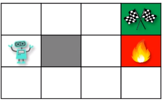
In the case of the minimalistic and discrete agent and environment depicted below, the state is the position of the agent in a grid world. In this world, there are a total of 11 different states. The action of the agent represents the movement of the agent into a neighbouring grid cell. There are a total of four different actions at the agent’s disposal. Not in all RL-systems are the states and actions discrete. Other systems possess continuous states or actions or both.
Basic Assumptions and Terminology
The following section describes some of the basic assumptions, terminology and equations used in reinforcement learning.
Reward Hypothesis
The reward hypothesis assumes that the goal of an intelligent agent is to maximise some sort of reward. The agent’s intelligence and all its capabilities are understood as being subservient to this goal.
Markov Property
The Markov Property assumes that an agent and its environment are memoryless. According to this property, the future state that an agent and environment will transition to depends only on the immediately preceding state and no other states further back in history.
Markov Decision Processes
The change of states due to the actions of an agent can be mathematically framed in terms of Markov Decision Processes (MDP). A MDP is a stochastic process that proceeds in discrete time steps. This process defines the probability of transitioning from one state to the next when taking an action and the associated reward.
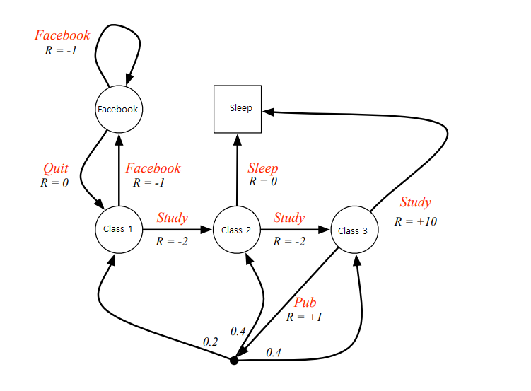
More information on Markov Decision Processes can be found for example in the article “Markov Decision Processes Simplified“.
Model-Free and Model-Based Reinforcement Learning
There exist two principle types of RL algorithms that differ from each other with respect to how they deal with state transition probabilities. A model-based RL algorithm tries to model these transition probabilities while a model-free RL algorithm does not. Therefore, a model-free RL algorithm is fully following a trial-and-error approach while a model-based RL algorithm does this to a lesser degree. All the RL algorithms explained in this article are model-free.
Policy
What an agent tries to learn in an RL-scenario is a policy that maximises reward. A policy defines the probability of an agent to take a certain action when the environment is in a certain state. The policy that maximizes the total reward is called the optimal policy. In mathematical equations, the policy is abbreviated as pi.
Policies can be implemented with any data structure and/or method that is suitable. For simple RL systems that operate on discrete states and actions, a policy can be implemented for example as a simple lookup table between states and actions. For more complicated RL systems with a large number or continuous states or actions, a policy can be implemented for example with a neural network. The same applies to state and value functions which are described further down.
On-Policy and Off-Policy Methods
In on-policy learning, the policy an agent uses to select actions is improved through learning. On-policy methods are called -greedy policies as they select random actions with an
probability and follow the optimal action with 1-
probability.
In off-policy learning, an optimal policy is discovered independently of the policy that an agent uses to select actions. Accordingly, these methods have two policies, a behaviour policy that is used for exploring and a target policy that is used for improvement.
On- and off-policy methods have their advantages and disadvantages. On-policy methods are said to be more stable and off-policy methods are more efficient and provide a better balance between the exploration of new policies and the exploitation of the currently best policies.
Discounted Cumulative Reward
In an RL system, not only the reward that an agent receives immediately after performing an action is important. Rather, an agent tries to maximise the accumulation of all rewards it receives from a particular point in time on until the end of what is called an episode (a simulation run). Typically, when summing these rewards, the influence of rewards that lie further in the future is made less strong than more immediate rewards. This is achieved by multiplying the rewards with a discount factor that is taken to the power of time. The discounted cumulative reward is mathematically defined as follows:

Value Functions
Value functions specify the return that can be expected by an agent when following its policy. There are two types of value functions, state value function and action value function.
State Value Function
The state value function is the expected return starting from the current state and then following a policy.

If states are discrete, state values are associated to all the states an agent and environment can be in. In case of the simple grid world example from before, the state values might assume the following values after a few training iterations:

An optimal state value function can be expressed in terms of the optimal policy:

Action Value Function
The action value function is the expected return starting from the current state, then taking an action, and then following a policy.

If both the states and actions are discrete, action values are associated with all state action pairs. In case of the simple grid world example from before, the action values might assume the following values after a few training iterations:

An optimal action value function can be expressed in terms of the optimal policy:

Bellman Equation
The Bellman equation decomposes a value function into two parts, the immediate reward plus the discounted future rewards. The second part can be formulated recursively.


These two equations can also can also be specified in terms of an optimal policy. In this case, the equations are named Bellman optimality equations.


TD-Error
TD in TD-Error stands for time difference. The TD-Error is frequently used in RL to improve the state or action value during learning. The TD-Error measures the difference between the currently observed state or action value and the previously assumed state or action value.
For the state value, the TD-Error is mathematically formulated as follows:

For the action value, the TD-Error is mathematically formulated as follows:

Using the TD-Error, the state or action values can be updated during training by adding to the current state or action value the corresponding TD-Error multiplied by the learning rate.


Example RL-Algorithm: SARSA
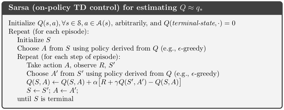
SARSA is a model-free on-policy method that works best with discrete states and actions. SARSA stands for the tuple S, A, R, S1, A1. S represents the current state, A the currently taken action, R the reward received after taking action A, S1 the next state, and A1 the next action taken. SARSA operates on action values. The pseudocode for training the SARA algorithm is as follows:
Example RL-Algorithm: Q-Learning
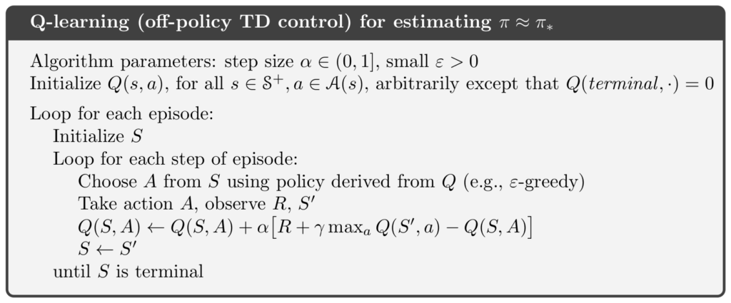
Q-Learning is a model-free off-policy method that also works best with discrete states and actions. Q-learning seeks to find the best action to take given the current state. Accordingly, the update function for the action value is slightly different from SARSA when it comes to selecting the action for the next state and action. Instead of selecting an action that is suggested by the current policy (as is the case with SARSA), the action chosen is the one whose action value is highest. The pseudocode for training the Q-Learning algorithm is as follows:
Policy Gradient Methods
Both SARSA and Q-Learning are value-based RL algorithm. Policy Gradient methods differ from value-based RL algorithms in that they operate directly on a policy instead of state or action value functions. Policy-based RL is effective in high dimensional and stochastic continuous action spaces and for learning stochastic policies. Value-based RL excels in sample efficiency and stability.
Many of the more sophisticated RL setups employ continuous states and actions. A classical example is the “MontainCar” simulation in which a car with a weak motor is located in a valley and needs to learn to accelerate back and forth to reach a mountain top.
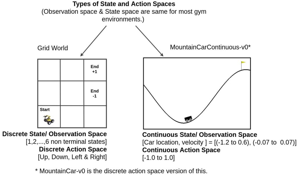
If the policy is represented by a parameterized function such as a neural network, then training consists of optimising these parameters to maximise the expected cumulative reward. The objective of maximising the expected cumulative reward can then formulated as follows:

Policy Gradient methods apply gradient ascent to maximise the objective. The gradient of the objective with respect to the parameters of the policy can be written as follows:

Updating the policy parameters during training then corresponds to:

The gradient can be rewritten using action probabilities of the parameterised policy function and parameterised action value function:

Actor-Critique Methods
Actor-Critique Methods employ both a policy function and a value function, both of them typically implemented as neural networks. The policy function is called the actor, the value function the critique. The actor decides which action to take, and the critic informs the actor how good the action taken was and how it should be adjusted. The term critique is reminiscent of the critique in Generative Adversarial Networks but its role is very different in Actor-Critique methods. In Actor-Critique methods, the actor and critique cooperate with each other and the both improve over time.

During training, instead of dealing with the expectation over the cumulative rewards of all possible trajectories, the cumulative rewards are only sampled from some trajectories. Furthermore, the action value function is replaced by an advantage function. An advantage function returns how much better (or worse) the reward for the currently chosen action is as compared with the current value function. For this reason, the advantage function is identical with the TD-Error.


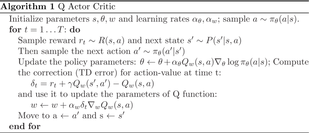
The pseudocode for training an Actor-Critique RL system is as follows:
